



Editorial Integrity
Making sound real estate investment decisions begins with reliable, data-driven insights. At Ziffy.ai, we offer an AI-native real estate investing, proprietary data-driven trend analysis, investment mortgage programs like DSCR loans, and a network of over 500 investor-friendly real estate agents to deliver the expertise needed for informed decisions. Our content is crafted by experienced real estate professionals and backed by real-time market data, ensuring you receive accurate and actionable information. Through a rigorous editorial process, we strive to empower your investment journey with trustworthy and up-to-date guidance.
Falling mortgage rates would help buyers, but in many U.S. markets they would not be enough.
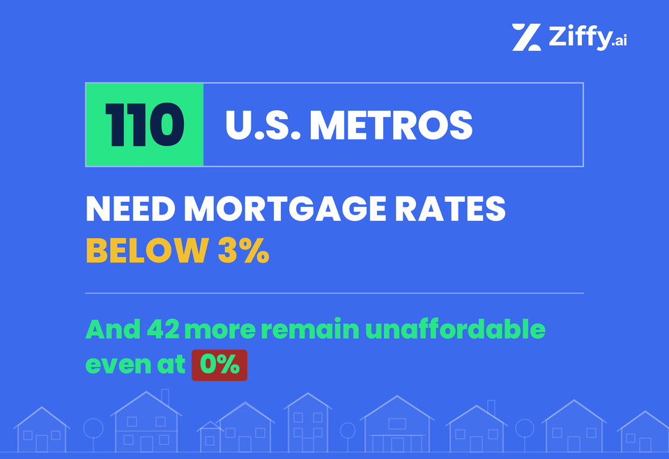
At the 6.49% benchmark, the median-priced listing is unaffordable for the median-income household in 316 of 364 metros analyzed. Even at 3%, 152 metros would remain above the modeled affordability threshold, including 42 where no nonnegative mortgage rate would close the gap.
The analysis defines affordability as total monthly housing costs equal to no more than 30% of median household income, assuming a 20% down payment, a 30-year mortgage, and standardized property tax and insurance costs.
Table of Contents
In Los Angeles, repaying mortgage principal alone costs about $2,444 a month against an affordability ceiling of $2,410
The median-priced listing is unaffordable even with 0% interest, $0 property tax and $0 homeowners insurance. The result also holds at the upper end of the ACS income range, where the threshold rises to approximately $2,435
152 metros, or 41.8%, require a mortgage rate below 3% or have no rate-only solution
Even at a 3% mortgage rate, more than two in five metros would remain above the modeled affordability threshold
At the 6.49% benchmark, 316 of 364 metros, or 86.8%, are unaffordable to the median-income household
Only 48 of 364 metros meet the modeled affordability threshold at 6.49%
Three in Four Metros Need Mortgage Rates Below 5% or Cannot Be Made Affordable Through Rate Reductions Alone
The 364 metros in the primary ranking divide into five groups based on the mortgage rate needed to make the median-priced listing affordable to the median-income household.
Mortgage-affordability outcome | Metros | Share of Primary Ranking |
|---|---|---|
Rates alone cannot restore affordability | 42 | 11.5% |
Needs a mortgage rate below 3% | 110 | 30.2% |
Needs a mortgage rate between 3.00% and 4.99% | 122 | 33.5% |
Needs a mortgage rate between 5.00% and below 6.49% | 42 | 11.5% |
Affordable at the | 48 | 13.2% |
Total | 364 | 99.9% |
Note: Shares do not sum to 100% because of rounding
The most severe group contains 42 metros with no positive mortgage-rate solution under the study’s standardized assumptions. Even if mortgage interest were reduced to 0%, repayment of the mortgage principal, standardized property tax and homeowners insurance would still exceed 30% of the median household’s gross monthly income.
Another 110 metros have a positive mathematical solution, but only at a mortgage rate below 3%. These metros are distinct from the no-solution group, although rates near 1% or 2% sit far outside the range usually contemplated in ordinary mortgage-rate forecasts.
A further 122 metros would require rates between 3.00% and 4.99%. Combined with the 110 sub-3% metros and the 42 with no rate-only solution, this means 274 of 364 metros, or 75.3%, either require a mortgage rate below 5% or cannot be made affordable through rate reductions alone.
The next 42 metros would cross the modeled affordability threshold at a rate between 5.00% and below 6.49%. This group is unrelated to the 42 metros with no rate-only solution despite the matching count.
The final 48 metros are already affordable at 6.49%, although the size of the cushion varies considerably. Baltimore–Columbia–Towson sits only 0.05 percentage points above the 6.49% threshold. For metros with unusually high theoretical break-even rates, the analysis describes them as “Affordable at 6.49% – substantial cushion” rather than publishing an uncapped modeled rate.
These categories are reporting bands, not economic cliffs. A metro requiring 2.99% is not meaningfully different from one requiring 3.01%. The analysis therefore publishes exact modeled rates and flags the 28 metros that fall within 0.10 percentage points of a band boundary.
Mortgage Rate Affordability in America Statistics [364 Metros Analyzed]
1. At the 6.49% Benchmark, the Median-Priced Listing Is Unaffordable to the Median-Income Household in 316 of 364 U.S. Metros
At Freddie Mac’s 6.49% average for the week ending July 9, 2026, 316 metros, or 86.8% of the primary ranking, exceed the study’s 30% housing-cost ceiling. Only 48 metros, or 13.2%, are affordable. The model includes principal and interest on an 80% mortgage, property tax equal to 1.1% of the listing price and homeowners insurance equal to 0.5%.
2. In 110 metros, mortgage rates would need to fall below 3%; in another 42, even a hypothetical 0% interest rate would not be enough
Together, these 152 metros account for 41.8% of the primary ranking. The first 110 have a positive mathematical solution below 3%. In the remaining 42, mortgage principal, standardized property tax and homeowners insurance already exceed 30% of median gross monthly household income at 0% interest. The zero-rate scenario is a mathematical test, not an available mortgage product.

Amresh Singh
Founder and CEO | Ziffy.ai
The same national mortgage rate produces very different affordability outcomes across markets. In some metros, a modest decline changes the result; in others, even eliminating interest does not close the gap.
3. In Los Angeles, repaying mortgage principal alone costs more than the median household can afford
Los Angeles has a median listing price of $1,099,950 and median household income of $96,405. With a 20% down payment, the modeled mortgage principal is $879,960. Dividing that principal across 360 monthly payments produces a principal-only payment of approximately $2,444, compared with an affordability ceiling of $2,410. The metro exceeds the threshold before interest, property tax or homeowners insurance is added, making the result independent of the study’s standardized recurring-cost assumptions.
4. Twenty of the 50 largest metros in the source dataset require a mortgage rate below 3% or have no rate-only solution
Fourteen of the 50 largest metros in the analysis require a mortgage rate below 3%, while six have no rate-only solution. Together, 20 metros or 40% fall into the two most severe categories. Fourteen of those 20 retain the same category across the ACS income range, while six change category and are treated as supplementary local examples. The six no-rate-only-solution metros are New York, Los Angeles, San Francisco, San Diego, San Jose and Providence-Warwick. Providence exceeds its modeled affordability threshold by about $60 a month at 0% interest, but its classification changes within the ACS income margin of error.
5. Only six of the 50 largest metros in the analysis are affordable at a 6.49% mortgage rate
Detroit, St. Louis, Baltimore, Pittsburgh, Cleveland and Buffalo are the only large metros where the median-priced listing fits within the 30% ceiling at 6.49%. Their modeled break-even rates are Pittsburgh (8.40%), St. Louis (7.71%), Detroit (7.53%), Buffalo (6.96%), Cleveland (6.80%) and Baltimore (6.54%). Baltimore sits only 0.05 percentage points above the 6.49% benchmark and changes category within the ACS income margin of error.
6. Los Angeles, San Francisco, San Diego and San Jose all have no positive rate-only solution despite California’s high metropolitan incomes
San Jose has median household income of $164,801, yet its $1,385,000 median listing costs approximately $4,924 a month at 0% interest against a $4,120 ceiling, a shortfall of $804. At 0% interest, San Diego remains approximately $575 above its ceiling, San Francisco approximately $153 above and Los Angeles approximately $1,501 above. High metropolitan incomes do not offset the scale of listing prices in these markets.
7. None of California’s 24 Eligible Metros Are Affordable at 6.49%
11 California metros have no rate-only solution, 12 require a mortgage rate below 3% and one, Hanford–Corcoran, requires a rate between 3% and 4.99%. The pattern extends inland. Riverside requires 0.77%, Stockton 0.93%, Fresno 1.00% and Sacramento 1.04%. California therefore has no eligible metro where the median-priced listing is affordable to the median-income household at 6.49% under the study’s standardized assumptions.
8. Miami requires a 1.36% mortgage rate, while Tampa and Orlando need rates above 3%
Miami’s median listing price is $499,000 against median household income of $80,625, producing a modeled break-even rate of 1.36%. Tampa requires 3.43% and Orlando 3.27%. All 22 eligible Florida metros are unaffordable at 6.49%, but the rate required varies sharply within the state. Miami sits in the ultra-low-rate category, while Tampa and Orlando would cross the modeled threshold at rates above 3%. Naples-Marco Island and Crestview–Fort Walton Beach–Destin have no rate-only solution under the central income estimate. Both change category within the ACS income margin of error and are therefore treated as supplementary rather than headline findings.
9. Indianapolis and San Antonio Are the Large Stable Metros Closest to Affordability at 6.49%
Indianapolis requires a mortgage rate of approximately 6.21%, only 0.28 percentage points, or 28 basis points, below the 6.49% benchmark. San Antonio requires approximately 5.76%, a decline of 0.73 percentage points, or 73 basis points. Birmingham has a smaller central gap at 6.23%, but its classification changes within the ACS income margin of error and should not lead the finding.
Other major metros requiring comparatively modest relief include Philadelphia (5.40%), Chicago (5.25%), Houston (4.98%), Minneapolis (4.88%), Washington, D.C. (4.52%), Atlanta (4.49%) and Dallas (4.25%). Indianapolis is the clearest major-metro example of a place where a relatively small rate decline would change the modeled outcome.
10. At a 5% mortgage rate, only 90 of the 364 metros would be affordable
A decline from 6.49% to 5.00% would add 42 metros to the affordable group, increasing the total from 48 to 90. The other 274 metros, or 75.3%, would still exceed the affordability ceiling. At 4%, 153 metros would be affordable. At 3%, the total would rise to 212, still leaving 152 metros beyond the threshold after a 3.49-percentage-point decline.
Metros With the Largest Monthly Affordability Gaps at 0% Interest
To identify markets where lower mortgage rates alone could not restore affordability, the analysis recalculated housing costs at 0% interest. This removes interest expense but still includes repayment of the borrowed principal, property taxes and homeowners insurance. In 42 metros, those remaining costs still exceed the modeled household budget.
Rank | Metro | Median | Median Household Income | Minimum Monthly Cost at 0% | Monthly | Gap |
|---|---|---|---|---|---|---|
1 | Santa Maria-Santa Barbara, CA | $1,747,250 | $95,637 | $6,212 | $2,391 | $3,822 |
2 | Salinas, CA | $1,236,250 | $93,290 | $4,396 | $2,332 | $2,063 |
3 | Santa Cruz-Watsonville, CA | $1,293,750 | $107,893 | $4,600 | $2,697 | $1,903 |
4 | Napa, CA | $1,397,000 | $122,754 | $4,967 | $3,069 | $1,898 |
5 | Los Angeles-Long Beach-Anaheim, CA | $1,099,950 | $96,405 | $3,911 | $2,410 | $1,501 |
6 | San Luis Obispo-Paso Robles, CA | $1,075,000 | $100,724 | $3,822 | $2,518 | $1,304 |
7 | Barnstable Town, MA | $909,450 | $87,925 | $3,234 | $2,198 | $1,035 |
8 | Kahului-Wailuku, HI | $999,000 | $101,168 | $3,552 | $2,529 | $1,023 |
9 | Bozeman, MT | $993,250 | $103,918 | $3,532 | $2,598 | $934 |
10 | San Jose-Sunnyvale-Santa Clara, CA | $1,385,000 | $164,801 | $4,924 | $4,120 | $804 |
Napa’s no-solution classification is stable. Its narrower principal-only result changes within the ACS income margin of error.
A metro’s position in this table is not a forecast of financial distress or a future price correction. It measures the standardized monthly affordability gap at the mathematical lower bound of mortgage interest.
San Jose shows that even the highest median household income estimate in the analysis may not offset an exceptionally high listing price. Its median household income of $164,801 is the highest of the 364 metros, and it is still $804 a month short at 0% interest.

Debjit Saha
Co-Founder and CTO | Ziffy.ai
A zero-interest test separates markets where lower rates could restore affordability from those where they cannot under the model. Once principal repayment and recurring costs already exceed the household budget, the problem is no longer the mortgage rate by itself.
Ten Metros Would Need Mortgage Rates Between 0.77% and 1.16%
The ranking is limited to metros whose reporting category remains stable across the ACS income margin-of-error range.
These metros have a positive mathematical solution but require the lowest rates among stable, headline-tier metros. No-solution metros are excluded from this ranking rather than being treated as if they required a 0% rate.
Among larger, heavily covered metros, Sacramento requires 1.04%, Nashville 1.54%, Portland 1.60%, Las Vegas 1.80%, Denver 2.72% and Phoenix 2.76%. These metros have positive mathematical solutions, but the required rates sit far below ordinary mortgage-market scenarios.
The Modeled Mortgage Rate Needed in Major U.S. Metros
The national mortgage rate conceals substantial variation among major metros. Metros are listed by size rather than ranked by affordability severity.
Note: Miami’s 1.36% modeled rate uses the report’s standardized 1.6% combined annual property-tax and insurance assumption. Its classification would change to no rate-only solution if the combined cost reached approximately 2.18% of the listing price.
Boston and Seattle are supplementary estimates. Their affordability category changes within the ACS household-income margin of error, and each would become no-solution after an increase of less than 0.04 percentage points in the combined annual tax-and-insurance assumption.
The table shows why saying mortgage rates need to fall is incomplete. Indianapolis needs a decline of 28 basis points and San Antonio 73 basis points. Chicago needs approximately 5.25%, Dallas and Austin approximately 4.25%, Phoenix and Denver approximately 2.7%, and Miami approximately 1.4%. New York and Los Angeles remain above the modeled affordability threshold even at 0% mortgage interest under the standardized assumptions.
A 5% Mortgage Rate Would Still Leave Three in Four Metros Unaffordable
The analysis recalculated affordability at seven mortgage-rate levels while holding listing prices, household incomes, the 20% down payment, the 30-year loan term, property taxes and homeowners insurance constant. Only the mortgage rate changes.
Mortgage Rate | Metros Affordable | Metros still unaffordable | Share Affordable |
|---|---|---|---|
6.49% | 48 | 316 | 13.2% |
6.00% | 56 | 308 | 15.4% |
5.00% | 90 | 274 | 24.7% |
4.00% | 153 | 211 | 42.0% |
3.50% | 175 | 189 | 48.1% |
3.00% | 212 | 152 | 58.2% |
0.00% | 322 | 42 | 88.5% |
A decline from 6.49% to 6% would move only eight additional metros below the modeled affordability threshold. At 5%, three in four would still remain unaffordable. Even at 3.5%, 189 of 364 metros would remain above the threshold. A majority does not cross the threshold until somewhere between the tested 3.5% and 3% scenarios.
Income-Lag Sensitivity
Household income data are from the 2024 American Community Survey, while listing prices are from June 2026. To test how possible nominal income growth since the ACS observation period could affect the headline results, the analysis increased every metro’s median household income by 3%, 5% and 8%, while holding listing prices and all financing assumptions constant.
| Income assumption | Metros requiring a rate below 3% | Metros with no nonnegative rate-only solution |
| Published 2024 ACS income | 110 | 42 |
| Income increased by 3% | 88 | 37 |
| Income increased by 5% | 87 | 30 |
| Income increased by 8% | 71 | 29 |
Note: The income increases are uniform sensitivity scenarios, not estimates of actual income growth in each metro. Local income changes may have been higher or lower.
Under the 8% sensitivity scenario, the two headline counts fall from 110 to 71 and from 42 to 29. The magnitude changes, but the direction of the finding does not: even after a uniform increase in household income, dozens of metros would still require mortgage rates below 3%, and 29 would remain beyond the reach of any nonnegative mortgage rate under the model.
The Modeled Price Gap Reaches 65.7% in Los Angeles and 36.7% in Miami
The analysis expresses the affordability gap in two ways: the mortgage-rate decline required if the listing price does not change, and the listing-price decline required if the mortgage rate stays at 6.49%.
Note: These figures measure the gap between the current median listing price and the maximum price affordable under the study assumptions. They are not forecasts of future price declines.
Metro | Rate needed | Rate decline | Median listing price | Affordable | Modeled |
|---|---|---|---|---|---|
Chicago-Naperville-Elgin, | 5.25% | 1.24 pp | $394,500 | $355,425 | 9.9% |
Houston-Pasadena-The Woodlands, TX | 4.98% | 1.51 pp | $362,265 | $318,801 | 12.0% |
Austin-Round Rock-San | 4.26% | 2.23 pp | $473,500 | $391,163 | 17.4% |
Dallas-Fort Worth-Arlington, | 4.25% | 2.24 pp | $439,990 | $363,111 | 17.5% |
Tampa-St. Petersburg-Clearwater, FL | 3.43% | 3.06 pp | $399,925 | $306,498 | 23.4% |
Orlando-Kissimmee-Sanford, | 3.27% | 3.22 pp | $419,990 | $317,341 | 24.4% |
Phoenix-Mesa-Chandler, | 2.76% | 3.73 pp | $489,500 | $352,930 | 27.9% |
Denver-Aurora-Centennial, | 2.72% | 3.77 pp | $589,000 | $423,072 | 28.2% |
Miami-Fort Lauderdale-West | 1.36% | 5.13 pp | $499,000 | $315,700 | 36.7% |
Los Angeles-Long Beach-Anaheim, CA | No positive solution | — | $1,099,950 | $377,489 | 65.7% |
Among no-solution metros the modeled gap runs wider still, reaching 78.6% in Santa Maria-Santa Barbara. Those metros are listed in the appendix.
Even if prices fell to these modeled thresholds, buyers would still need suitable homes to be available at that level. An earlier analysis of starter-home inventory found that sub-$300,000 listings had disappeared in 42 U.S. markets and accounted for less than 1% of inventory in another 13, illustrating why lower prices on paper do not always translate into homes buyers can actually find.
These modeled gaps are not forecasts of future price declines or estimates of what sellers would accept.
They provide a second measurement of the same gap. If rates do not fall to the modeled break-even level, affordability would require lower listing prices, greater household resources or different financing assumptions.
Among 48 Affordable Metros, These 10 Have the Largest Modeled Price Cushions
The median-priced listing meets the modeled affordability threshold in 48 metros. The ranking below shows the 10 stable metros with the largest affordable-price cushions, measured as a share of the median listing price.
Among the 50 largest metros in the analysis, Detroit, St. Louis, Baltimore, Pittsburgh, Cleveland and Buffalo are affordable at the 6.49% benchmark, although Baltimore changes category within the ACS income margin of error.
Many of the largest affordability cushions appear in the Midwest, Appalachia and parts of the South. The findings apply to the median-income household under the study assumptions, not to every buyer or property.
Note: The full list of 48 affordable metros is available upon request.
In Five California Metros, the Modeled Affordable Price Is at Least 65% Below the Median Listing Price
The table includes stable, headline-tier metros, ranked by the percentage difference between the current median listing price and the modeled affordable price. Where no mortgage rate can restore affordability, the analysis calculates the maximum listing price affordable at 6.49% benchmark. These are modeled affordability gaps, not forecasts of future price declines.
Note: The metros are ranked by modeled price gap as a percentage of the current median listing price, from largest to smallest.
Metro | Current median listing price | Affordable price | Dollar gap | Modeled price gap |
|---|---|---|---|---|
Santa Maria–Santa Barbara, CA | $1,747,250 | $374,482 | $1,372,768 | 78.6% |
Salinas, CA | $1,236,250 | $365,292 | $870,958 | 70.5% |
Santa Cruz–Watsonville, CA | $1,293,750 | $422,472 | $871,278 | 67.3% |
Los Angeles-Long Beach-Anaheim, CA | $1,099,950 | $377,489 | $722,461 | 65.7% |
Napa, CA | $1,397,000 | $480,663 | $916,337 | 65.6% |
Note: Affordable price is the maximum modeled listing price at 6.49%, including for metros with no positive rate-only solution at their current median listing price.
Some Major-Metro Results Are More Sensitive to Local Ownership Costs Than Others
The central ranking applies the same 1.1% property-tax and 0.5% homeowners-insurance assumptions to every metro. These standardized assumptions allow consistent comparisons but may differ materially from local costs. They are likely to understate property taxes in parts of Illinois and Texas and insurance costs in parts of Florida.
A separate sensitivity test calculates how far the combined recurring-cost rate could rise or fall before each selected major metro changes classification.
Chicago, Dallas, Houston and Miami should be interpreted as standardized comparisons rather than localized borrower estimates. Higher actual tax or insurance costs would reduce the mortgage rate those markets could support.
- Los Angeles remains a no-rate-only-solution metro even if property tax and homeowners insurance are reduced to zero.
- New York remains in the no-solution category unless combined annual property tax and insurance fall below approximately 1.12% of the listing price.
- Miami would move from requiring a 1.36% mortgage rate to having no nonnegative rate-only solution if combined annual property tax and insurance reached approximately 2.18% of the listing price.
- Boston and Seattle are the most fragile major-metro estimates. Boston would change classification if recurring costs increased by approximately $148 a year, while Seattle would change after an increase of approximately $298. Both are also income-sensitive and should be treated as supplementary rather than headline findings.
Note: Dallas, Houston, Chicago, Austin, Tampa and Orlando have substantially more headroom under the standardized assumptions. Full sensitivity results are available in the methodology workbook.
How ACS Income Uncertainty Affects the National Counts
The central findings use each metro’s published ACS median household-income estimate. As a conservative uncertainty test, the analysis also recalculated the national counts with every metro’s income set simultaneously to the lower and upper ends of its ACS margin-of-error range.
Under this test, the number of metros unaffordable at 6.49% ranges from 304 to 330, compared with the central estimate of 316. The number requiring a mortgage rate below 3% ranges from 86 to 134, while the no-rate-only-solution count ranges from 29 to 56. The combined number requiring a sub-3% rate or having no rate-only solution ranges from 115 to 190, compared with the central estimate of 152.
These are conservative bounds, not a national confidence interval. They place every metro at the same end of its income range simultaneously and should not be interpreted as a standard error or probability range.
| National finding | Central estimate | Lower-income bound | Higher-income bound |
| Unaffordable at 6.49% | 316 | 330 | 304 |
| No rate-only solution | 42 | 56 | 29 |
| Requires below 3% | 110 | 134 | 86 |
| Below 3% or no solution | 152 | 190 | 115 |
Methodology
Data Sources
This analysis uses three primary data inputs.
1. Median listing prices and active listing counts
Realtor.com Research monthly metro-level housing data supplied the June 2026 median listing price, the June 2026 active listing count, and the CBSA codes and metro names used throughout. Realtor.com’s research data covers MLS-listed residential properties and publishes monthly housing metrics for U.S. metros and other geographic levels.
Median listing price refers to the asking price of the median active listing, not the median sale price or an estimate of the price at which a property ultimately closes. It may also change because the composition of active inventory changes, for example, if a greater share of higher-priced or lower-priced homes enters the market. It should therefore not be interpreted as a pure measure of underlying home-price appreciation or decline.
2. Median household income
Median household income came from the U.S. Census Bureau’s 2024 American Community Survey 1-year estimates, table B19013, which reports median household income in the past 12 months in 2024 inflation-adjusted dollars. The analysis used the income estimate, its associated 90% margin of error, and metropolitan and micropolitan statistical area geographies.
3. Current mortgage-rate benchmark
The mortgage-rate benchmark is Freddie Mac’s Primary Mortgage Market Survey average for a 30-year fixed-rate mortgage. This report uses Freddie Mac’s 6.49% average for the week ending July 9, 2026, and all rate-dependent findings are anchored to that observation. Because Freddie Mac publishes PMMS weekly, subsequent survey rates may differ from the benchmark used in this analysis.
Metros Included in the Analysis
The analysis matched 393 metros with both housing and income data. The primary ranking includes 364 stateside metros with at least 200 active listings.
The 29 excluded records are:
- 6 Puerto Rico metros, excluded on geography;
- 23 stateside metros with 100 to 199 active listings, classified as low inventory and excluded from the primary ranking.
Three of the six Puerto Rico metros have fewer than 100 active listings. Because all three are already excluded on geography, the sub-100 listing floor removes no additional stateside metro from the primary ranking.
The 200-listing threshold is a reporting-quality screen rather than a formal confidence interval. It is intended to reduce the influence of unusually thin active inventory, but it does not establish statistical representativeness or imply that every included metro is measured with equal precision.
ACS 1-year estimates are published only for areas with populations of 65,000 or more, so metros dropping out at the source stage are concentrated among smaller metros. All 100 of the largest metros identified in the source dataset are present.
How Affordability Was Defined
The analysis applies the same financing and recurring-cost assumptions to every metro:
- 20% down payment;
- 80% mortgage;
- 30-year fixed-rate term;
- property tax equal to 1.1% of the listing price annually;
- homeowners insurance equal to 0.5% of the listing price annually; and
- a modeled affordability threshold equal to 30% of gross monthly household income.
The model excludes mortgage insurance, homeowners association fees, maintenance and repairs, utilities, closing costs, buyer debt obligations, lender-specific qualification rules, and mortgage points or other upfront rate-buydown costs.
For each metro:
Modeled affordability threshold = Median household income × 30% ÷ 12
Mortgage amount = Median listing price × 80%
Monthly property tax = Median listing price × 1.1% ÷ 12
Monthly homeowners insurance = Median listing price × 0.5% ÷ 12
The modeled monthly housing cost equals monthly principal and interest plus monthly property tax and monthly homeowners insurance. A metro is classified as affordable at a given mortgage rate when that total is less than or equal to the modeled affordability threshold.
The 30% threshold is used as a standardized housing-cost benchmark for comparison. It should not be interpreted as a lender approval standard or as a claim that households spending more than 30% of income are necessarily unable to purchase a home.
Note: These standardized assumptions are designed for consistent metro-to-metro comparison. They are not property-level underwriting estimates.
How the Mortgage Rate Needed Was Calculated
For each currently unaffordable metro, the analysis solves for the mortgage rate at which:
Monthly principal and interest + standardized monthly tax + standardized monthly insurance = 30% of median gross monthly household income
Because total monthly cost rises monotonically with the mortgage rate, the solution is unique. The rate is solved numerically rather than estimated from rounded payment tables.
Metros are then placed into reporting categories:
| Modeled outcome | Definition |
|---|---|
| Rates alone cannot restore affordability | The modeled cost exceeds the affordability ceiling even at 0% interest |
| Needs below 3% | Modeled rate needed is less than 3.00% |
| Needs 3.00% to 4.99% | Modeled rate needed is at least 3.00% and below 5.00% |
| Needs 5.00% to below 6.49% | Modeled rate needed is at least 5.00% and below 6.49% |
| Affordable at 6.49% | The modeled break-even rate is equal to or above 6.49%, or the modeled housing cost at 6.49% is already within the affordability threshold. |
These categories are reporting bands, not economic cliffs. A metro requiring 2.99% is not materially different from one requiring 3.01%. The analysis therefore also publishes exact modeled rates and flags metros within 0.10 percentage points of 3%, 5% or the 6.49% benchmark.
How No-Solution Metros Were Identified
A metro has no rate-only solution when the modeled monthly cost exceeds the affordability ceiling even at 0% interest. At 0% the household still repays the 80% mortgage principal over 360 months and still pays standardized property tax and insurance:
Monthly principal repayment at 0% = Mortgage amount ÷ 360
The 0% scenario is a mathematical lower-bound test, not an available mortgage product. It isolates whether mortgage interest is the binding affordability constraint.
The analysis also calculates a narrower principal-only test that excludes tax and insurance. It identifies metros where repayment of mortgage principal alone exceeds 30% of median gross monthly household income. This test is reported separately and is not identical to the broader no-solution classification. A metro may be stable under the category test while its principal-only result changes within the ACS income margin of error.
How Affordable Prices and Price Gaps Were Calculated
The analysis calculates the maximum listing price affordable at the benchmark mortgage rate. Because the mortgage amount, property tax and homeowners insurance all change with the listing price, the affordable price is solved as the price at which total modeled monthly housing cost equals the modeled affordability threshold.
Modeled price gap = (Current median listing price − Affordable price) ÷ Current median listing price
Affordable-price cushion = (Affordable price − Current median listing price) ÷ Current median listing price
Each measure is floored at zero, so a metro reports either a price gap or a price cushion, never a negative value of the other.
These figures are standardized affordability comparisons. They are not forecasts of future home-price declines, estimates of market value or predictions of what sellers would accept.
Mortgage-Rate Scenarios
The analysis recalculates affordability across all 364 metros at 6.49%, 6.00%, 5.00%, 4.00%, 3.50%, 3.00% and 0.00%, counting at each rate the metros that meet the affordability threshold, the metros that remain above it, and the affordable share of the primary ranking.
Scenario counts are reported only at these tested rates. The analysis does not interpolate between them.
The scenarios hold listing prices, household incomes, the down payment and standardized recurring-cost assumptions constant. They isolate the effect of changing the mortgage rate rather than forecasting how prices or incomes might respond.
Income-Lag Sensitivity
The central analysis uses 2024 ACS median household income because it is the income vintage available for the metro universe used in the study. To test the effect of possible nominal income growth between the ACS observation period and June 2026, the analysis also recalculates all classifications after increasing every metro’s median household income by 3%, 5% and 8%, while holding listing prices and all other assumptions constant.
These scenarios are uniform sensitivity tests, not estimates of actual income growth in each metro. Local income changes may have been higher or lower.
Income Uncertainty and Publication Tiers
ACS median household income is published with a 90% margin of error. To test whether a metro’s reporting category is sensitive to income uncertainty, the analysis recalculates the mortgage rate needed using the central estimate, the central estimate minus the margin of error, and the central estimate plus the margin of error.
Two tests are applied in order. A metro is first checked for a category change across the income range. Only metros that keep the same category are then checked against the size of their margin.
| Income-sensitivity status | Definition |
|---|---|
| Category Stable | Keeps the same reporting category across the income range, and the margin of error is 10% or less of the income estimate |
| Changes category under income MOE | Moves into a different reporting category at the low or high end of the income range |
| High uncertainty | Keeps the same reporting category across the income range, but the margin of error exceeds 10% of the income estimate |
Of the 364 metros in the primary ranking, 222 retain the same reporting category across the full ACS income margin-of-error range and have an income margin of error of 10% or less. Another 128 change category within that range, while 14 retain their category but have a margin of error above 10%.
Because the category test runs first, a metro with a wide margin that also changes category is reported as changes category, not high uncertainty. Thirty-three metros in the primary ranking have an ACS income margin of error above 10% of the central estimate. Nineteen of those already change reporting category across the income range and are classified accordingly; the remaining 14 are classified as high uncertainty.
Within the 42 no-solution metros, 26 are category stable. Within the 110 metros requiring a rate below 3%, 55 are category stable.
Category-stable metros form the primary headline publication tier. The report’s ranked top-ten tables use category-stable metros. Supplementary major-metro tables may include income-sensitive markets, which are marked directly beside the estimate.
Boston and Seattle fall into the “Changes category under income MOE” group and should be treated as supplementary examples rather than headline-tier findings.
Local Tax-and-Insurance Sensitivity
The central analysis applies a combined annual property-tax and homeowners-insurance cost equal to 1.60% of the listing price: 1.10% for property tax and 0.50% for insurance. The same assumption is used nationwide to support consistent metro comparisons.
This limitation is especially relevant for prominent findings in Texas, Illinois and Florida, where actual property-tax or homeowners-insurance costs may differ materially from the standardized national assumptions. Results for metros including Miami, Dallas, Houston, Chicago, Tampa and Orlando should therefore be read alongside the sensitivity analysis rather than as locally customized borrower estimates.
In the main report, these metros are marked with the note: “Standardized national tax-and-insurance assumption; see sensitivity notes.”
Because actual local costs vary, the analysis also calculates how high the combined tax-and-insurance burden could rise before a metro’s result changes. For each of the 15 headline metros, the analysis calculates:
- the combined annual cost rate at which the mortgage rate needed would fall below 3%;
- the combined annual cost rate at which no mortgage-rate reduction could restore affordability.
The difference between each threshold and the central 1.60% assumption is reported as headroom. Smaller headroom means the result is more sensitive to local tax and insurance costs. Negative headroom means the metro would cross the relevant threshold even if recurring costs were below the standardized assumption.
Both thresholds are calculated directly from the same listing-price, income, down-payment, mortgage-term and affordability assumptions used in the central model. They are exact within the model but still depend on its financing and affordability assumptions, and they do not replace locally verified property-level tax or insurance quotes. The 15 headline metros were selected before the sensitivity results were reviewed.
Limitations
- Listing prices are not transaction prices: Realtor.com median listing prices measure active asking prices, not closed-sale prices or appraised values.
- Point-in-time housing data: The analysis uses June 2026 listing conditions. Inventory composition and median listing prices change over time.
- Income timing: Housing data is from June 2026, while income comes from the 2024 ACS. The analysis does not adjust metro incomes forward to 2026.
- Median-to-median comparison: The median-priced listing is compared with the median-income household. The household earning the median income is not necessarily purchasing the median-priced property.
- Standardized tax assumption: Actual property-tax rates vary substantially by state, municipality, property type, exemptions and assessed value. The uniform 1.1% assumption may understate or overstate local costs.
- Standardized insurance assumption: Actual homeowners insurance varies by location, property characteristics, coverage and risk exposure. The uniform 0.5% assumption may understate or overstate local costs.
- Excluded housing expenses: HOA fees, mortgage insurance, maintenance, utilities, closing costs and buyer debt are not included.
- Down-payment assumption: The model assumes a 20% down payment. A smaller down payment would increase the mortgage balance and may add mortgage insurance. A larger down payment would reduce the monthly payment but require more upfront cash.
- No credit or underwriting model: The analysis does not account for credit score, debt-to-income requirements, reserves, loan limits, lender overlays or individual borrower eligibility.
- No behavioral response: Rate scenarios hold prices and incomes constant. They do not model how lower rates could affect buyer demand, listing prices, inventory or household earnings.
- Metro-level results: Affordability can vary widely within a metro. The analysis should not be used to evaluate a specific neighborhood, property or borrower.
- Inventory floor: The 200-listing requirement improves comparability but does not eliminate all sampling volatility.
- ACS sampling uncertainty: Median household income is an estimate. Metro findings that change category within the ACS margin of error should be interpreted cautiously.
- 0% scenario: A 0% mortgage is not presented as a commercially available product. It is a mathematical test of whether interest-rate reductions alone can restore affordability.
- Rate comparability: Freddie Mac’s PMMS represents a national conventional conforming purchase-loan average for a specific borrower and property profile. Actual rates vary by credit, loan size, occupancy, property type, points and lender.
Technical Notes and Replicability
Definitions
| Term | Definition |
|---|---|
| Median-priced listing | The June 2026 median listing price reported for the metro by Realtor.com |
| Median-income household | The 2024 ACS 1-year median household income estimate for the matched metro geography |
| Affordable monthly housing cost | 30% of median gross monthly household income |
| Down payment | 20% of the median listing price |
| Mortgage amount | 80% of the median listing price |
| Mortgage term | 30 years, or 360 monthly payments |
| Benchmark mortgage rate | Freddie Mac’s 6.49% average 30-year fixed rate for the week ending July 9, 2026 |
| Standardized property tax | 1.1% of the listing price annually |
| Standardized homeowners insurance | 0.5% of the listing price annually |
| Mortgage rate needed | The annual mortgage rate at which modeled monthly housing cost equals 30% of median gross monthly household income |
| No rate-only solution | The modeled monthly cost exceeds the affordability ceiling even at 0% interest |
| Affordable at 6.49% | The mortgage rate needed is at or above 6.49% |
| Affordable price at 6.49% | The maximum listing price that fits within the affordability ceiling at a 6.49% mortgage rate under the same assumptions |
| Price cushion | The amount by which the affordable price exceeds the current median listing price |
| Modeled price gap | The percentage by which the current median listing price exceeds the affordable price at 6.49% |
| Headroom | The difference between a metro’s combined tax-and-insurance break-even threshold and the standardized 1.60% assumption |
| Basis point | One-hundredth of one percentage point; 100 basis points equals 1 percentage point |
Mortgage Payment Formula
Monthly principal and interest for positive mortgage rates:
Monthly principal and interest = P × [r(1 + r)ⁿ] ÷ [(1 + r)ⁿ − 1]
Where P is the mortgage amount, r is the annual mortgage rate divided by 12, and n is 360 monthly payments.
At 0% interest, principal repayment is the mortgage amount divided by 360.
Rate Display Rules
The break-even-rate calculation is not capped. In a small number of low-priced metros, the median-income household could service the median-priced listing at a rate well above any plausible mortgage market.
Two reporting rules apply:
- a separate published-rate field is capped at 15% for display purposes;
- exact break-even rates above 10% are not published, because presenting a metro as able to absorb a 12% or 14% mortgage would be unrealistic and distracting.
Six metros in the primary ranking have a modeled rate above 10%. They are reported as affordable with a substantial cushion, expressed through the modeled affordable price rather than an exact rate. The highest modeled rate in the primary ranking is 13.66%, so the 15% display cap does not bind on any published metro; it applies only to lower-inventory metros held in the underlying data.
Affordable-price and price-cushion figures are computed directly from the payment equation and do not depend on the break-even-rate estimate.
Geographic Matching
Realtor.com housing records and ACS income records were matched on CBSA code, which both sources publish. Codes are unique within the dataset, and no metro appears twice.
Metro display names follow the Realtor.com convention. Because Realtor.com and Census title the same CBSA differently in some cases, names were standardized for presentation only. Name text was not used to establish the match.
Only records with a housing-to-income match on CBSA code were retained. A crosswalk of Realtor.com metro name, Census metro name, CBSA code and match status is available on request.
Aggregation and Ranking Approach
National counts are metro counts, not household-weighted, population-weighted or listing-weighted estimates. Each of the 364 metros contributes one observation to statistics such as the number and share affordable at 6.49%, the number requiring a rate below 3%, the number with no rate-only solution, and the number affordable at each tested rate.
The analysis therefore describes the share of included metros meeting each condition. It does not estimate the share of U.S. households or homebuyers affected.
Metro-level rankings use the metric named in each table: monthly shortfall at 0%, mortgage rate needed, modeled price gap, affordable-price cushion, or metro size for the selected major-metro table.
Quality-Control Steps
- confirmed that every primary-ranking metro met the 200-active-listing floor;
- confirmed that all national category counts summed to 364;
- recalculated displayed shares from unrounded counts;
- confirmed that rate-band classifications matched each metro’s exact modeled rate;
- separately identified no-solution metros and metros with a positive rate solution;
- verified that no-solution metros carry no rate value rather than a zero;
- checked mortgage-rate declines in both percentage points and basis points;
- recalculated affordability at each selected scenario rate;
- checked price-gap and price-cushion calculations against unrounded values;
- tested category stability using the ACS income margin of error;
- flagged modeled rates within 0.10 percentage points of a reporting boundary;
- suppressed exact break-even rates above 10% in published tables;
- recomputed every metro against an independent implementation of the payment and solver formulas and reconciled the results;
- reviewed major-metro and state-level claims against the underlying metro records.
Displayed dollar values, percentages and rates are rounded for readability. Calculations and classifications use unrounded values.
Replicability
To reproduce the central calculation for a metro:
- Obtain the metro’s June 2026 median listing price and active listing count from Realtor.com Research.
- Confirm that the metro has at least 200 active listings.
- Obtain the metro’s 2024 ACS 1-year median household income estimate and margin of error from table B19013, matching on CBSA code.
- Calculate the monthly affordability ceiling: median household income × 30% ÷ 12.
- Calculate the mortgage amount: median listing price × 80%.
- Calculate monthly property tax: median listing price × 1.1% ÷ 12.
- Calculate monthly homeowners insurance: median listing price × 0.5% ÷ 12.
- Calculate monthly principal and interest at the mortgage rate being tested using a 360-month fixed-rate amortization schedule.
- Add principal and interest, property tax and homeowners insurance.
- Compare the total with the monthly affordability ceiling.
- To calculate the mortgage rate needed, numerically solve for the rate at which modeled housing cost equals the affordability ceiling.
- To test for no rate-only solution, set interest to 0% and calculate principal repayment as the mortgage amount divided by 360.
- Repeat using income plus and minus the ACS margin of error to test category stability.
Notes
- All metro counts and shares use the 364-metro primary ranking unless otherwise stated.
- Shares may not sum to exactly 100% because displayed percentages are rounded.
- Rates, dollar amounts and basis-point changes are displayed in rounded form, while calculations use unrounded values.
- A metro requiring 2.99% is not economically distinct from one requiring 3.01%; reporting bands are used for communication rather than as natural economic breakpoints.
- “No rate-only solution” means no mortgage rate at or above 0% restores affordability under the standardized assumptions. It does not mean that no combination of a lower purchase price, larger down payment, higher income or different cost assumptions could restore affordability.
- Major metros are selected for editorial relevance and are ordered by metro size rather than by affordability severity.
- Additional metro records, sensitivity results and low-inventory observations are available upon request at contact@ziffy.ai.
About Ziffy
Ziffy is an AI-native real estate investment platform that helps investors discover, analyze, and finance U.S. real estate opportunities. The platform combines property search, investment analysis, and access to specialized financing solutions, including DSCR, fix-and-flip, and bridge loans. This research was produced by Ziffy’s data analytics team to provide transparency into housing, lodging, and affordability trends.