





Editorial Integrity
Making sound real estate investment decisions begins with reliable, data-driven insights. At Ziffy.ai, we offer an AI-native real estate investing, proprietary data-driven trend analysis, investment mortgage programs like DSCR loans, and a network of over 500 investor-friendly real estate agents to deliver the expertise needed for informed decisions. Our content is crafted by experienced real estate professionals and backed by real-time market data, ensuring you receive accurate and actionable information. Through a rigorous editorial process, we strive to empower your investment journey with trustworthy and up-to-date guidance.
Mortgage rates often dominate the housing-affordability debate, but financing costs are only one part of the equation. A companion Ziffy analysis calculated the mortgage rate each metro would need to meet a standardized affordability threshold. This report approaches the question from the other direction: holding the mortgage rate at 6.67%, how far below current home values do standardized income-affordability and asking-rent parity benchmarks sit?
For each metro, Ziffy calculates two standardized benchmarks: an income-affordability benchmark based on median household income and an asking-rent parity benchmark based on local ZORI asking rents. The analysis uses the lower of the two as a conservative stress-test reference point.
The modeled gap measures the percentage decline from the current typical single-family home value needed to reach that lower benchmark under the study’s assumptions. The lower benchmark is not an estimate of fair value, and the modeled gap is not a forecast of future home-price declines.
About the 20% threshold: The 20% level is an analytical reporting threshold used to compare metros consistently. It is not an industry definition of overvaluation, a forecast trigger, or a level at which the model predicts home prices will decline.
Table of Contents
Every Covered Metro Exceeds the 20% Threshold in Six State Groups; None Do in Nine
Among the 34 Zillow-assigned states with at least four covered metros, every covered metro has a modeled decline-to-benchmark gap greater than 20% in California, Oregon, Idaho, Utah, Montana and Massachusetts under the baseline assumptions. Nine qualifying states including Ohio, Illinois and Iowa have no covered metro above the threshold.
Lower rates reduce the modeled gap, but do not eliminate it in every market
A 50-basis-point reduction in the standardized mortgage rate lowers the number of metros above the 20% modeled-gap threshold from 139 to 112. Even at an illustrative 4.67% rate, 64 covered metros remain above the threshold.
San Jose has the highest median household income among covered metros, yet its modeled decline-to-benchmark gap is 63.4% under the baseline assumptions.
All 25 covered metros assigned to California exceed the 20% modeled-gap threshold in the baseline model, with a median gap of 40.3%.
Assumption sensitivity: The count above 20% ranges from 106 to 183 under the tested tax-and-insurance assumptions. It falls to 112 at a 6.17% rate and to 109 when every metro’s 2024 income estimate is increased by an illustrative 8%.
Nearly 3 in 4 Covered Metros Have a Positive Modeled Gap
At a standardized 6.67% mortgage rate, the lower modeled benchmark sits below the June 2026 typical single-family home value in 280 of 375 covered U.S. metros, or 74.7%. The table below groups all covered metros by the size of the modeled decline-to-benchmark gap.
Modeled outcome | Metros | Share |
|---|---|---|
At or below both supported levels | 95 | 25.3% |
Greater than 0% and up to 10% | 65 | 17.3% |
Greater than 10% and up to 20% | 76 | 20.3% |
Greater than 20% and up to 30% | 63 | 16.8% |
Greater than 30% and up to 40% | 37 | 9.9% |
Greater than 40% | 39 | 10.4% |
Total | 375 | 100.0% |
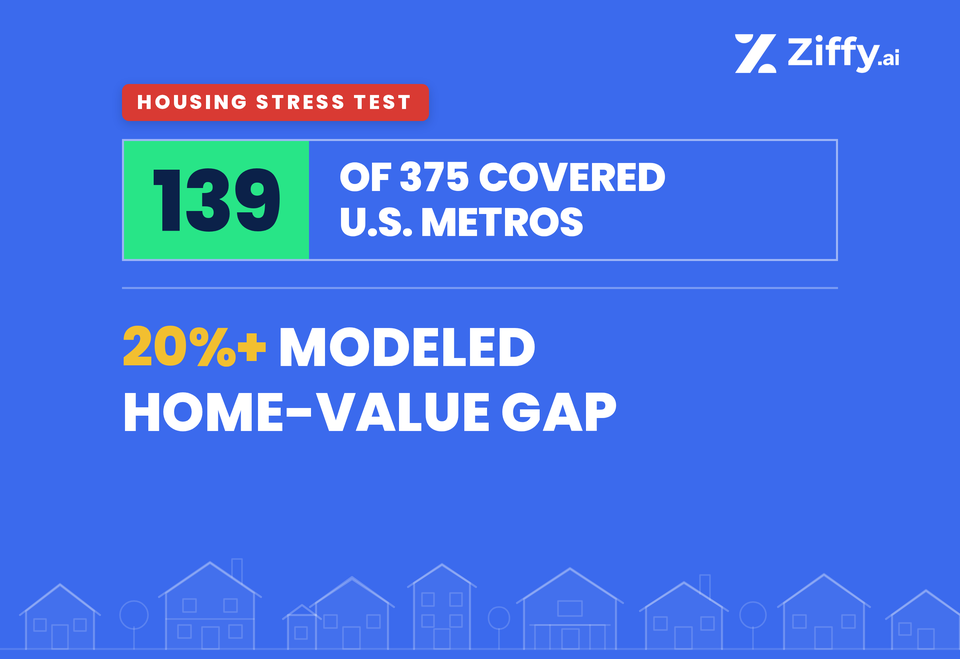
Overall, 139 metros, or 37.1% of the covered universe, have a modeled decline-to-benchmark gap greater than 20%. In 39 metros, the gap exceeds 40%.
Note: Bands use unrounded modeled gaps. The headline 20% and 40% counts use strict greater-than thresholds.
Why This Matters
The findings do more than show that housing is expensive. Applying the same stress test across 375 metros makes it possible to compare the size of the gap consistently across markets and test whether those results survive changes in key assumptions.
The analysis also shows that large modeled gaps can coexist with rising home values. Among the 39 metros with baseline gaps greater than 40%, 21 still recorded year-over-year home-value growth. That distinction is important: the model measures affordability and rent-parity stress, not where home prices are likely to move next.
Together, these findings show that large modeled affordability gaps can persist across different assumptions without functioning as a simple signal of where home prices will move next.
10 Key Findings From the 375-Metro Housing Stress Test
1. At the 20% Gap Threshold, 122 Metros Breach the Income-Affordability Benchmark, 87 the Asking-Rent Parity Benchmark, and 70 Both
Typical home values are above the lower of the two modeled benchmarks in 280 of 375 covered metros, or 74.7%. The remaining 95 metros are at or below both benchmarks. At the 20% modeled-gap threshold, 122 metros have an income-affordability gap greater than 20%, 87 have an asking-rent parity gap greater than 20%, and 70 exceed the threshold under both calculations. Because the reported modeled gap uses whichever benchmark is lower, 139 metros have an overall modeled gap greater than 20%.
Test at the 20% threshold | Metros |
|---|---|
Income-affordability gap greater than 20% | 122 |
Asking-rent parity gap greater than 20% | 87 |
Both gaps greater than 20% | 70 |
Overall modeled gap greater than 20% | 139 |
2. 104 Metros Remain Above the 20% Threshold Across Every Core Sensitivity Test
Of the 139 metros above the 20% modeled-gap threshold under the baseline assumptions, 104 remain above it under every predefined core one-at-a-time sensitivity scenario.“Scenario-stable” does not mean statistically certain; it means the metro remains above the threshold under each specified test. The sensitivity analysis is designed to show how dependent the baseline classifications are on changes to key model assumptions.
3. Modeled Decline-to-Benchmark Gaps Exceed 20% in 139 Metros and 40% in 39
The modeled gap is greater than 20% in 139 metros, greater than 30% in 76, and greater than 40% in 39. Among the 280 metros with a positive modeled gap, the median gap is 19.9%. These thresholds are reporting categories rather than sharp economic dividing lines. Fourteen metros sit within one percentage point of the 20% threshold, while 40 cross the threshold in at least one scenario using the ACS household-income estimate’s margin of error. The 139 figure should therefore be treated as a baseline model classification, not as a statistically exact national count or a prediction that home values will decline.

Amresh Singh
Founder and CEO | Ziffy.ai
Lower rates reduce the modeled gap, but the tested rate changes do not eliminate it in every market. Income, rent, property taxes and insurance also influence the result.
4. Under the Baseline Assumptions, Every Covered Metro Exceeds the 20% Gap Threshold in Six State Groups; None Do in Nine
Among the 34 Zillow-assigned states with at least four covered metros, every covered metro has a modeled gap greater than 20% in California, Oregon, Utah, Montana, Idaho, and Massachusetts under the baseline assumptions. Nine qualifying states have no covered metro above the threshold: Ohio, Indiana, Illinois, Louisiana, Iowa, Minnesota, Kentucky, Kansas, and Oklahoma. The remaining 19 qualifying states fall between those outcomes. The highest shares are concentrated in California and several Western states, while a group of interior states has no covered metro above the threshold. These are unweighted results among covered metros assigned to each Zillow state label, not statewide estimates. Multistate metros are assigned to one state and may not reflect conditions across their full geographic footprint.
5. The 10 Steepest Annual Home-Value Declines Split Evenly Above and Below the 20% Threshold
Across all 375 covered metros, larger modeled gaps were associated with slower year-over-year home-value growth overall, but individual markets moved in both directions. Some of the steepest annual declines occurred in lower-gap markets, including Punta Gorda, with a 7.6% decline and a 10.4% modeled gap, and Cape Coral, with a 6.0% decline and an 8.8% gap. Others occurred in higher-gap markets, including Naples, with a 4.5% decline and a 45.3% gap; Kahului, with a 3.6% decline and a 63.8% gap; and Stockton, with a 3.4% decline and a 33.3% gap. Of the 10 metros with the steepest annual declines, five were above the 20% modeled-gap threshold and five were below. The modeled gap measures distance from the two standardized benchmarks and should not be interpreted as a short-term price-direction or market-timing signal.

Debjit Saha
Co-Founder and CTO | Ziffy.ai
The two benchmarks answer different questions. In the largest-gap markets, the income-supported benchmark usually sets the lower ceiling. In many lower-gap markets, the gross-rent benchmark is lower. The binding label identifies which standardized test is stricter; it does not identify the cause of local housing conditions.
6. Home Values Still Rose in 21 of 39 Metros With Baseline Gaps Above 40%
A large modeled gap does not necessarily coincide with falling home values. Among the 39 metros with baseline modeled gaps greater than 40%, 21 recorded positive year-over-year home-value growth and 18 recorded declines. Median growth for the group was approximately 0.2%. Metros above the 20% threshold grew more slowly than those at or below it, with median annual growth of 0.84% versus 2.67%. The fact that home values were still rising in more than half of the metros with gaps above 40% underscores that the modeled gap is not a short-term price-direction signal or a forecast that home values will decline.
Note:Technical correlation statistics are reported separately in the methodology rather than treated as validation of the model.
7. Income Affordability Is the Lower Benchmark in 64 of 76 Metros With Gaps Above 30%
The asking-rent parity benchmark is lower in 61 of the 95 metros with no positive modeled gap. Among the 76 metros with modeled gaps greater than 30%, the pattern reverses: the income-affordability benchmark is lower in 64. In most of the largest-gap markets, the benchmark based on 30% of median household income produces a lower modeled home value than the asking-rent parity calculation. In many lower-gap markets, the asking-rent parity benchmark is the stricter of the two. The lower, or “binding,” benchmark identifies only which test is mathematically stricter under the model. It does not establish the cause of local housing conditions or account for factors such as housing supply, migration, zoning, new construction, buyer wealth, or household composition.
8. Los Angeles Has a 63.9% Decline-to-Benchmark Gap; Houston Has No Positive Gap
Among 25 large covered metros ordered by Zillow SizeRank, Los Angeles has a 63.9% baseline decline-to-benchmark gap. In other words, the lower modeled benchmark is 63.9% below its June 2026 typical single-family home value under the baseline assumptions. Other large modeled gaps include San Diego at 58.3%, San Francisco at 57.7%, New York at 49.4%, Miami at 45.4%, Seattle at 44.8%, and Boston at 42.3%.
At the other end, Houston has no positive modeled gap under the same assumptions. Dallas has a modeled gap of 3.1%, Detroit 5.6%, and Chicago 8.0%. The mortgage-rate assumption is identical across these markets. The differences reflect the local relationship among typical single-family home values, median household income, and typical asking rent.
Metro | June 2026 typical SFR value | Modeled gap | Lower benchmark | ZHVI YoY |
|---|---|---|---|---|
New York, NY | $761,300 | 49.4% | Income affordability | +4.2% |
Los Angeles, CA | $1,030,504 | 63.9% | Income affordability | +0.9% |
Chicago, IL | $380,637 | 8.0% | Income affordability | +4.6% |
Houston, TX | $312,512 | 0.0% | Income affordability | -2.0% |
Miami, FL | $569,830 | 45.4% | Income affordability | -1.4% |
Phoenix, AZ | $457,183 | 23.9% | Income affordability | -1.6% |
Denver, CO | $599,059 | 30.4% | Income affordability | -2.6% |
Washington, DC | $631,408 | 22.9% | Income affordability | -0.3% |
Note: Zillow SizeRank is used only to select and order this large-metro comparison. It is not a ranking by modeled gap.
9. Santa Cruz Has the Largest Baseline Point Estimate; California Accounts for 11 of the Top 25
Santa Cruz has the largest baseline point estimate at 65.6%, followed closely by Santa Maria at 65.5% and Los Angeles at 63.9%. California accounts for 11 of the 25 largest baseline point estimates, more than any other state. Hawaii, Oregon, and Montana each account for two of the top 25. Arizona, Massachusetts, Wisconsin, Nevada, Colorado, New York, Washington, and Idaho each account for one.
The income-affordability benchmark is lower in 24 of the 25 markets. Sheboygan, Wisconsin, is the only exception, with the asking-rent parity benchmark setting the lower modeled value. Three top-25 metros have comparatively wide ACS household-income margins of error: Flagstaff, where the margin equals 11.7% of the estimate; Carson City, at 19.2%; and Corvallis, at 11.4%. Their exact rankings should therefore be interpreted with additional caution.
Ranking note: Rankings reflect baseline point estimates. Differences between nearby metros have not been tested for statistical significance, and rank order may change within ACS household-income margins of error.
Note: Metro display names follow Zillow’s labels. Official CBSA names and codes are included in the downloadable dataset.
10. The 20% Count Falls From 139 to 105-128 Under Illustrative Income Adjustments
The model uses 2024 ACS household income alongside June 2026 home values and asking rents. Because the income data are from an earlier period, the analysis tests how the results change when every metro’s household-income estimate is increased by the same illustrative percentage. An 8% illustrative increase reduces the number of metros above the 20% modeled-gap threshold from 139 to 109 and lowers the median modeled gap from 19.9% to 17.4%.
Illustrative income adjustment | Metros above 20% |
|---|---|
+3% | 128 |
+5% | 118 |
+8% | 109 |
+10% | 105 |
Under the 8% scenario, 30 metros move below the 20% threshold, showing that the precise national count is sensitive to the income vintage.
The broad Western concentration remains visible, but some state-level results change. California falls from 25 of 25 covered metros above the threshold to 23 of 25, while Massachusetts falls from 5 of 5 to 3 of 5. Idaho, Montana, Oregon, and Utah continue to have every covered metro above the threshold.
Note:These adjustments are illustrative sensitivity scenarios, not sourced estimates of 2026 household income.
The 25 Largest Modeled Gaps
Ranked by the baseline modeled decline-to-benchmark gap between the June 2026 typical single-family home value and the lower of the two standardized benchmarks.
Most Stretched Markets
Note:Rankings reflect baseline point estimates only. Nearby ranks should not be interpreted as statistically distinct. ACS income uncertainty and changes in model assumptions may alter the ordering or threshold classification of individual metros.
Results for 25 Large Covered Metros, Ordered by Zillow SizeRank
Twenty-five large covered metros ordered by Zillow SizeRank, showing the modeled decline-to-benchmark gap, binding benchmark, annual home-value change and listing price-cut share.
Largest Metros
Note: Home-value and rent inputs use Zillow’s single-family series. Listing indicators use the all-homes series covering houses and condominiums.
State-Label Results Among Covered Metros
Share of each state’s covered metros with a baseline modeled gap greater than 20%, along with the state’s median modeled gap.
State Summary
Note:Limited to states with at least four covered metros. State assignment follows Zillow’s single-state label; multistate metros are attributed to one state.
How Modeled Gaps Compare With Recent Home-Value Declines
Recent home-value movement varies substantially across metros with similar modeled gaps. Of the 10 covered metros with the steepest year-over-year declines, five were above the 20% modeled-gap threshold and five were below. This reinforces that the modeled gap is a cross-sectional stress-test measure, not a short-term price forecast.
Metro | ZHVI change, June 2025–June 2026 | Modeled Gap | Listings with a price cut, June 2026 |
|---|---|---|---|
Punta Gorda, FL | -7.6% | 10.4% | 23.5% |
Cape Coral, FL | -6.0% | 8.8% | 24.2% |
Austin, TX | -5.7% | 17.5% | 28.4% |
North Port, FL | -5.3% | 25.2% | 27.1% |
Sherman, TX | -4.9% | 10.5% | 29.4% |
Naples, FL | -4.5% | 45.3% | 20.9% |
Kahului, HI | -3.6% | 63.8% | 16.9% |
Asheville, NC | -3.6% | 32.3% | 24.6% |
Elizabethtown, KY | -3.5% | 0.0% | 27.5% |
Stockton, CA | -3.4% | 33.3% | 26.0% |
Methodology
The results use June 2026 Zillow single-family home values and ZORI asking rents, 2024 American Community Survey median household income, a standardized 6.67% mortgage rate, and the financing and carrying-cost assumptions described below.
The analysis uses June 2026 Zillow single-family home values and ZORI asking rents, 2024 ACS median household income, a standardized 6.67% mortgage rate, and the financing and carrying-cost assumptions described below.
Timing of inputs: The analysis applies an August 2026 financing rate to June 2026 housing values and asking rents. The 2024 ACS income estimate is the latest available annual metro household-income measure. Because these inputs do not come from the same period, the report includes income and mortgage-rate sensitivity tests to show how the results change under alternative assumptions.
Data Sources
1. Typical home value: Zillow Home Value Index (ZHVI), single-family homes, smoothed and seasonally adjusted, June 2026. ZHVI represents the typical home value in a market for homes roughly in the 35th to 65th percentile of the value distribution. It is not a median sale-price or transaction-price series; the findings therefore refer to home values, not home prices.
2. Typical rent: Zillow Observed Rent Index (ZORI), single-family residences, smoothed and seasonally adjusted, June 2026. ZORI is a repeat-rent index weighted to the rental housing stock and reflects asking rents.
3. Median household income: U.S. Census Bureau American Community Survey 2024 one-year estimates, table B19013. The analysis uses estimate B19013_001E and margin of error B19013_001M, matched to each metropolitan statistical area by Core Based Statistical Area code. The 2024 estimates reflect data collected from January through December 2024.
4. Standardized mortgage rate: Freddie Mac Primary Mortgage Market Survey 30-year fixed average of 6.67% for the week ending August 13, 2026. PMMS reflects a conventional, conforming, owner-occupied, single-family purchase-loan profile with good-to-excellent credit and a 20% down payment. It is not an investor, DSCR, jumbo, or borrower-specific mortgage quote.
5. Listing indicators: The share of listings with a price cut, days to pending, and for-sale inventory come from Zillow’s monthly market data, using the June 2026 smoothed all-homes series covering houses and condominiums. These indicators are analyzed separately from ZHVI and ZORI, which use single-family series.
6. Data timing: Metro-level Census income data are published annually, 2024 ACS is the latest available income vintage used in this analysis. This is paired with June 2026 Zillow home-value and rent data. The analysis applies Freddie Mac’s 6.67% average 30-year fixed mortgage rate for the week ending August 13, 2026.
The analysis uses Zillow’s smoothed listing series. These figures may differ from Zillow’s unsmoothed monthly headline statistics.
Metros Included in the Analysis
The analysis began with 894 Zillow region rows carrying a June 2026 single-family ZHVI observation.
The 519 excluded records comprise:
- 305 regions without a single-family ZORI rent series.
- 120 Zillow regions without a confirmed 2024 ACS metropolitan match.
- 94 micropolitan areas, which fall outside the study’s metropolitan scope.
The final study universe contains 375 metropolitan statistical areas with all three required inputs:
- A June 2026 single-family ZHVI value.
- A June 2026 single-family ZORI rent estimate.
- A matched 2024 ACS one-year median household income estimate.
The rent-series requirement not population rank, is the largest filter. Only 589 of the 894 source regions carry a single-family ZORI observation. Geographic classification and ACS matching reduce the final universe to 375.
Because inclusion depends on Zillow rent-series availability and geographic matching, the 375 metros are a coverage universe rather than a random or population-weighted sample of U.S. housing markets. National counts in this report therefore refer only to the 375 covered metros.
ACS one-year estimates are available for every official metropolitan statistical area. The 120 unmatched Zillow regions were excluded because a confirmed 2024 ACS metropolitan match could not be established. They were not excluded because an official MSA fell below a 65,000-person ACS publication threshold.
Two Zillow regions that initially failed name-based matching were restored after a code-level review confirmed their CBSA assignments:
- The Villages, Florida, matched to the Census geography “Wildwood–The Villages.”
- California, Maryland, matched to the Census geography “Lexington Park.”
The geographic scope covers the 50 states and the District of Columbia. Puerto Rico is outside the study scope. The crosswalk ledger contains 900 rows: 894 Zillow source-region records used in the coverage funnel and six Puerto Rico MSA documentation rows added for completeness. The six Puerto Rico rows are not part of the 894-record Zillow source universe.
Every source region and its disposition including CBSA code, Census name, metro or micro classification, inclusion status, exclusion reason, match method, and manual override is recorded in the accompanying crosswalk and exclusion ledger.
How the Modeled Gap Was Calculated
The model applies the same financing and recurring-cost assumptions to every metro:
- 20% down payment.
- 80% loan-to-value ratio.
- 30-year fixed mortgage.
- 6.67% annual mortgage rate.
- Property tax equal to 1.1% of home value annually.
- Homeowners insurance equal to 0.5% of home value annually.
- Housing costs limited to 30% of gross monthly household income.
The 1.1% property-tax and 0.5% homeowners-insurance rates are uniform, analyst-selected assumptions used to make the metro results comparable. They are not estimates of each metro’s actual tax or insurance costs and should not be interpreted as official national averages.
Using uniform tax and insurance assumptions improves comparability across metros but reduces local realism; actual carrying costs can differ materially by location and property.
The 30% threshold follows the conventional housing-cost affordability standard commonly used by HUD. In this analysis, it is applied specifically to modeled principal, interest, property tax, and homeowners insurance. It is not a complete mortgage-qualification test.
For each metro, the model calculates two supported home-value levels.
Income-affordability benchmark: The home value at which modeled monthly principal, interest, property tax and homeowners insurance equal 30% of median gross monthly household income.
Asking-rent parity benchmark: The home value at which Zillow’s typical monthly ZORI asking rent equals those same modeled monthly ownership costs.
The model intentionally uses the lower of the two benchmarks so that a metro must satisfy both the income-affordability and asking-rent parity tests. This is a conservative analytical choice, not a standard valuation rule or a claim that the lower benchmark represents market value.
The gross-rent-supported calculation excludes:
- Vacancy.
- Repairs and routine maintenance.
- Capital expenditures.
- Property management.
- Leasing costs.
- HOA fees.
- Owner-paid utilities.
- Transaction costs.
- Required debt-service coverage.
- Required return on equity.
The asking-rent parity benchmark is therefore not an investor DSCR calculation, estimate of landlord profitability or investor valuation.
The model reports the lower of the two benchmarks. This creates a deliberately strict stress test in which a metro must satisfy both the income-affordability and asking-rent parity calculations. Choosing the lower benchmark is an analyst-selected methodological rule; it is not a standard industry valuation method and does not imply that the lower benchmark represents market value.
Key Formula
The monthly-cost-per-dollar-of-value factor, k, combines mortgage principal and interest with property tax and homeowners insurance:
k = LTV × [i(1 + i)ⁿ ÷ ((1 + i)ⁿ − 1)] + (tax + insurance) ÷ 12
where LTV is 0.80, i is the annual mortgage rate divided by 12, and n is 360 monthly payments. At a 6.67% mortgage rate, with property tax equal to 1.1% of value and homeowners insurance equal to 0.5%, k equals 0.0064796. This means every $1,000 of permitted monthly housing cost supports approximately $154,300 of home value.
Income-affordability benchmark = (30% × annual median household income ÷ 12) ÷ k
Asking-rent parity benchmark = typical monthly gross rent ÷ k
Lower modeled benchmark = minimum of the income-supported and Asking-rent parity benchmark
Modeled gap = max(0, 1 − lower benchmark ÷ current typical home value)
Because current home value is the denominator, a 20% modeled gap means the lower benchmark is 20% below the current value. It does not mean the current value is 20% above the benchmark.
A home value at or below both supported levels receives a modeled gap of zero. Holding all other inputs fixed, the modeled gap is mathematically equivalent to the percentage value decline that would place the current typical value at the Lower modeled benchmark. It is not a forecast that such a decline will occur.
Because property tax and insurance are modeled as percentages of home value, both costs decline proportionally when the standard model solves for a lower Modeled benchmark. Actual tax assessments and insurance premiums may not adjust in the same way.
Worked Example: Los Angeles
The following example uses rounded values for Los Angeles:
| Input or result | Value |
|---|---|
| June 2026 typical single-family home value | $1,030,504 |
| 2024 median household income | $96,405 |
| June 2026 typical monthly single-family rent | $4,506 |
| Income-affordability benchmark | $371,953 |
| Asking-rent parity benchmark | $695,334 |
| Lower modeled benchmark | $371,953 |
| Modeled gap | 63.9% |
Interpretation: Under the baseline assumptions, the lower modeled benchmark is 63.9% below the June 2026 typical single-family home value. This is equivalent to the modeled percentage decline from the current value required to reach that benchmark; it does not mean the current value is 63.9% above the benchmark.
Mortgage-Rate, Income, Rent, and Cost Scenarios
The report tests how the results change when key assumptions are varied. Unless otherwise stated, each sensitivity changes one input while holding the others constant.
Income vintage
The model combines 2024 household income with June 2026 home values and rents. Where household income increased after 2024, the older estimate may overstate the modeled gap relative to a contemporaneous-income comparison. The direction and magnitude vary by metro.
Increasing every metro’s income estimate by an illustrative amount produces the following results:
| Illustrative income adjustment | Metros above the 20% threshold |
| No adjustment | 139 |
| +3% | 128 |
| +5% | 118 |
| +8% | 109 |
| +10% | 105 |
Under the illustrative 8% adjustment, the median modeled gap among metros with a positive gap declines from 19.9% to 17.4%.
These adjustments are not sourced estimates of 2026 household income.
Mortgage rate
| Standardized mortgage rate | Metros above the 20% threshold |
| 4.67% | 64 |
| 6.17% | 112 |
| 6.67% | 139 |
| 7.17% | 161 |
These scenarios show how the modeled gap responds to specified mortgage-rate changes. They do not estimate future mortgage rates or future home values.
Property tax and homeowners insurance
The standard calculation uses combined annual property tax and homeowners insurance equal to 1.6% of home value.
| Combined annual tax and insurance | Metros above the 20% threshold |
| 1.2% | 106 |
| 1.6% | 139 |
| 2.2% | 183 |
The wide range reflects the material effect of carrying-cost assumptions. Actual tax and insurance expenses vary substantially by state, metro, property, insurer, and borrower.
Scenario-stable count
Of the 139 metros above the 20% threshold under baseline assumptions, 104 remain above it under every scenario in the predefined core one-at-a-time sensitivity set. “Scenario-stable” means the result survives each specified scenario individually; it is not a statistical confidence interval or probability statement.
- Income at the ACS estimate plus and minus its margin of error.
- Income increased by 3% and 5%.
- Rent increased and decreased by 5%.
- Mortgage rate increased and decreased by 50 basis points.
- Combined tax and insurance of 1.2% and 2.2%.
- Sticky-insurance treatment.
“Scenario-stable” means that a metro remains above the threshold under each scenario in this predefined set. It is not a statistical confidence classification.
Combined favorable scenario
Applying the following assumptions simultaneously leaves 71 metros above the 20% threshold:
- Mortgage rate reduced to 6.17%.
- Household income increased by 5%.
- Typical rent increased by 5%.
- Combined annual property tax and insurance reduced to 1.2%.
This is an illustrative combined scenario, not a forecast or estimate of the most favorable plausible outcome.
Sticky-insurance scenario
The standard calculation assumes homeowners-insurance expense declines proportionally with the modeled home value.
The sticky-insurance scenario instead holds each metro’s current-dollar homeowners-insurance expense constant when solving for the Modeled benchmark. This tests the possibility that insurance premiums would not decline alongside home values.
ACS income uncertainty
The ACS publishes a 90% margin of error for each metro income estimate. Recalculating the model at the upper and lower income bounds produces the following classification changes:
- 93 metros switch which supported level is lower.
- 27 switch between a positive modeled gap and no positive modeled gap.
- 40 cross the 20% reporting threshold in at least one income-bound scenario.
Metros whose income margin of error exceeds 10% of the income estimate are flagged. Flagstaff, Carson City, and Corvallis meet this condition in the top-25 table and remain included with an explicit uncertainty flag.
Threshold proximity
Two separate proximity checks are used:
- Zero-gap boundary: Ten metros sit within one percentage point of the point at which the current value equals the Lower modeled benchmark.
- Twenty-percent reporting threshold: Fourteen metros sit within one percentage point of the 20% threshold.
These deterministic scenarios and proximity checks are not forecasts, probability ranges, confidence intervals for the full model, or estimates of best- and worst-case outcomes.
Limitations
- Typical value, not sale price: ZHVI is an index of typical home value, not a median transaction, listing, or appraised price.
- Not a valuation or forecast: The modeled gap measures distance from two specified supported levels under fixed assumptions. It is not an estimate of intrinsic value, market-clearing value, future sale price, or the amount by which values are expected to decline.
- Not a complete affordability index: The model uses median household income and typical gross rent. It does not measure every factor affecting housing affordability or market value, including supply, employment, migration, construction, zoning, buyer wealth, credit availability, or transaction costs.
- Not mortgage qualification: The income-supported calculation does not account for household debt, credit score, down-payment availability, closing costs, mortgage points, private mortgage insurance, HOA fees, maintenance, utilities, lender overlays, or other underwriting requirements.
- Income timing: Income is measured in 2024, while home values and rents are measured in June 2026. Using the older income estimate may overstate the modeled gap where incomes subsequently increased. The direction and magnitude vary by metro.
- Median-to-typical comparison: The median-income household is not necessarily purchasing the typical single-family home represented by ZHVI.
- Uniform carrying-cost assumptions: The 1.1% property-tax and 0.5% insurance rates are standardized assumptions rather than local estimates. They may understate or overstate actual costs in specific markets.
- Cost scaling: The standard calculation assumes property tax and insurance decline proportionally with the modeled value. In practice, assessments may adjust with a delay and insurance premiums may not decline when values fall.
- Gross rent is not net income: The Asking-rent parity benchmark excludes vacancy, repairs, management, capital expenditures, HOA expenses, owner-paid utilities, leasing costs, transaction expenses, debt-service coverage requirements, and return on equity.
- Value and rent composition: Single-family ZHVI and single-family ZORI do not necessarily represent the same properties, bedroom counts, quality tiers, or neighborhoods. Differences between the owner and rental housing stocks may affect the rent-to-value comparison.
- Gross yield is not independent validation: Rent and home value are inputs to both gross rental yield and the modeled gap. A relationship between the two measures is therefore partly mechanical.
- Equal metro weighting: Every covered metro counts once regardless of population, housing stock, number of households, or transaction volume. National metro counts are not population-weighted estimates of U.S. households or homes.
- Data-availability selection: Inclusion requires a single-family ZORI observation and a confirmed ACS metropolitan match. Excluded markets may differ systematically from included markets, and the 375 covered metros are not a random sample.
- Listing indicators use a different property universe: Price-cut share, days to pending, and inventory use Zillow’s all-homes series covering houses and condominiums. ZHVI and ZORI use single-family series.
- Listing indicators do not measure distress: A price reduction can reflect an aspirational initial list price, routine seller strategy, changing competition, or market conditions. Price-cut share is not a direct measure of seller distress or completed transactions.
- Mortgage-rate comparability: The 6.67% PMMS rate represents a conventional owner-occupied borrower profile. It is not an investor, DSCR, jumbo, or borrower-specific rate.
- Metropolitan scope: The analysis covers metropolitan statistical areas only. Micropolitan areas are excluded by design.
- State-label summaries: State results are unweighted summaries of covered metros assigned to one Zillow state label. They are not statewide estimates, and multistate metros may be represented under only one state label.
- Within-metro variation: Values, rents, incomes, taxes, and insurance expenses can vary substantially within a metropolitan area. The results should not be used to evaluate an individual neighborhood, property, borrower, or investment.
- Source revisions: Zillow may revise historical index values. The findings are tied to the exact files and download timestamp documented in the source manifest.
- Correlation does not establish causality: The reported correlations are descriptive, unadjusted cross-sectional relationships. They do not establish that the modeled gap causes slower or faster home-value growth. The modeled gap and annual ZHVI-change calculation also both use current ZHVI as an input.
Technical Notes and Replicability
Definitions
| Term | Definition |
| Typical home value | June 2026 single-family ZHVI, smoothed and seasonally adjusted; a typical value for homes roughly in the 35th to 65th percentile, not a median sale price |
| Typical rent | June 2026 single-family ZORI, smoothed and seasonally adjusted; a stock-weighted repeat-rent measure of typical asking rent |
| Median household income | 2024 ACS one-year median household income estimate for the matched CBSA |
| Standardized mortgage rate | Freddie Mac’s 6.67% average 30-year fixed rate for the week ending August 13, 2026 |
| Modeled monthly cost | Principal and interest on an 80% mortgage, plus property tax and homeowners insurance |
| Income-affordability benchmark | The home value at which modeled monthly cost equals 30% of median gross monthly household income |
| Asking-rent parity benchmark | The home value at which typical monthly gross rent equals modeled monthly cost |
| Lower modeled benchmark | Whichever of the income-supported and Asking-rent parity benchmark is lower for a metro |
| Modeled gap | The resulting percentage is called the modeled decline-to-benchmark gap. It measures the percentage decline from the current typical home value that would be required to reach the lower modeled benchmark while holding the model’s assumptions constant. It is a fixed-assumption stress test not a forecast, appraisal, estimate of market value or prediction that home values will decline by that amount. |
| Cost-per-dollar factor, (k) | Modeled monthly cost per $1 of home value; 0.0064796 under the standard assumptions |
| Basis point | One-hundredth of one percentage point; 100 basis points equal one percentage point |
| Covered metro | A metropolitan statistical area with a June 2026 single-family ZHVI value, June 2026 single-family ZORI estimate, and matched 2024 ACS income estimate |
Quality-Control Steps
The analysis underwent the following checks:
- Coverage and crosswalk reconciliation: Confirmed that 375 included metros and 519 exclusions accounted for all 894 Zillow source-region records and reviewed every rent-present exclusion at the CBSA-code level.
- Duplicate and geography checks: Confirmed that no metro or CBSA code appeared more than once and reviewed the two manual aliases used for The Villages, Florida, and California, Maryland.
- Formula recomputation: Recomputed every metro’s cost factor, Income-affordability benchmark, Asking-rent parity benchmark, Lower modeled benchmark, and modeled gap through a separate implementation of the formulas.
- Threshold and reporting reconciliation: Verified all reporting bands, threshold counts, lower-level classifications, displayed shares, and major tables using unrounded values.
- Sensitivity and uncertainty testing: Reran the mortgage-rate, income, rent, carrying-cost, sticky-insurance, combined favorable, and ACS margin-of-error scenarios.
- Statistical and editorial verification: Confirmed the correlation results and reviewed the major-metro, top-25, state-label, and threshold claims against the underlying records. The mortgage-rate date, Zillow observation month, ACS vintage, model version, article tables, and downloadable files were also checked for consistency.
Across all 375 metros, the modeled gap and year-over-year ZHVI change had a Spearman rank correlation of (ρ = -0.312), with (p < 0.001).
Across the 373 metros with complete price-cut observations, the modeled gap and listing price-cut share had a Spearman rank correlation of (ρ = 0.013), with (p = 0.80).
Displayed dollar amounts, home values, rents, percentages, rates, and correlation statistics are rounded for readability. All calculations and classifications use unrounded values.
Replicability
To reproduce the central calculation for a metro:
- Obtain the June 2026 single-family ZHVI value and single-family ZORI rent estimate from Zillow Research.
- Obtain the 2024 ACS one-year median household income estimate and margin of error from table B19013, matching the metro by CBSA code.
- Set the standardized assumptions:
- Mortgage rate: 6.67%.
- Loan-to-value ratio: 80%.
- Mortgage term: 360 months.
- Annual property-tax rate: 1.1%.
- Annual homeowners-insurance rate: 0.5%.
- Income housing-cost threshold: 30%.
- Calculate the monthly mortgage rate:
i = 6.67% ÷ 12 - Calculate the monthly cost-per-dollar factor:
k = 0.80 × [i(1 + i)^360 ÷ ((1 + i)^360 − 1)] + 1.6% ÷ 12 - Calculate the monthly income-based housing-cost limit:
median household income × 30% ÷ 12 - Calculate the Income-affordability benchmark:
(median household income × 30% ÷ 12) ÷ k - Calculate the Asking-rent parity benchmark:
monthly gross rent ÷ k - Take the lower of the income-supported and asking-rent parity benchmark
- Calculate the modeled gap:
max(0, 1 −lower modeled benchmark÷ current typical home value) - Record whether the income-supported or asking-rent parity benchmark is lower.
- To test income uncertainty, repeat the calculation using the ACS income estimate plus and minus its published margin of error.
Notes
- All metro counts and shares use the 375-metro study universe unless otherwise stated.
- Shares may not total exactly 100% because displayed percentages are rounded.
- Calculations use unrounded source values even when tables display rounded amounts.
- A metro with a 19.9% modeled gap is not economically distinct from one at 20.1%. Reporting thresholds are communication categories, not natural economic breakpoints.
- The Lower modeled benchmark identifies which of the two standardized calculations is mathematically stricter. It does not identify the economic cause of local housing conditions.
- Home-value and rent inputs use Zillow’s single-family series. Listing indicators use Zillow’s all-homes series covering houses and condominiums.
- Large-metro comparisons are selected and ordered using Zillow SizeRank. Zillow SizeRank is used for editorial comparison and is not a ranking by modeled gap.
- State-label summaries use Zillow’s assigned state for each metro and are not population-weighted statewide estimates.
- The modeled gap may narrow through changes in home values, incomes, rents, mortgage rates, property taxes, insurance expenses, or a combination of those factors.
- Additional metro records, the full crosswalk ledger, and sensitivity results are available upon request at contact@ziffy.ai.
About Ziffy
Ziffy is an AI-native real estate investment platform that helps investors discover, analyze, and finance U.S. real estate opportunities. The platform combines property search, investment analysis, and access to specialized financing solutions, including DSCR, fix-and-flip, and bridge loans. This research was produced by Ziffy’s data analytics team to provide transparency into housing, lodging, and affordability trends.