





Editorial Integrity
Making sound real estate investment decisions begins with reliable, data-driven insights. At Ziffy.ai, we offer an AI-native real estate investing, proprietary data-driven trend analysis, investment mortgage programs like DSCR loans, and a network of over 500 investor-friendly real estate agents to deliver the expertise needed for informed decisions. Our content is crafted by experienced real estate professionals and backed by real-time market data, ensuring you receive accurate and actionable information. Through a rigorous editorial process, we strive to empower your investment journey with trustworthy and up-to-date guidance.
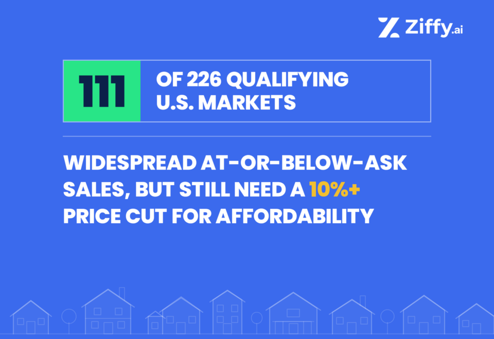
At-or-below-ask sales are widespread across many qualifying U.S. housing markets, but that does not necessarily mean homes are affordable.
In 111 of 226 qualifying U.S. study markets, at least two-thirds of single-family homes sold at or below their original asking price in August 2026. Yet even at those closed-sale prices, the median home still required an additional modeled reduction of at least 10% to meet the study’s affordability threshold.
The gap is considerably larger in 93 markets, where the median closed-sale price would need to be at least 20% lower in the model to meet that threshold. Of those 93 markets, 60 also had at least two-thirds of homes selling at or below original ask.
This analysis compares August 2026 Redfin single-family closed-sale data with estimated household income and modeled ownership costs at Freddie Mac’s 6.95% September 17 mortgage-rate benchmark. Overall, 197 of 226 qualifying markets remained above the modeled affordability threshold.
Table of Contents
All 21 covered Florida markets fall into the headline cohort
Every qualifying Florida market combines widespread at-or-below-ask sales with a modeled affordability gap of at least 10%, and the median required reduction across those markets is 24.9%.
Every one of the 16 covered California markets needs a modeled price reduction of at least 20% to reach the affordability threshold
But only nine also have at least two-thirds of homes selling at or below original ask showing that severe affordability pressure does not always come with widespread at-or-below-ask sales.
Texas shows the opposite pattern: all 17 covered markets pass the at-or-below-ask gate, but only 10 still need a modeled reduction of 10% or more
Houston has 90.1% of homes selling at or below original ask but requires only an 8.3% modeled reduction, while San Antonio is at 91.7% and 4.7%.
At-or-Below-Ask Frequency and Housing Affordability Are Not the Same Thing
The study measures two separate conditions. The first is how frequently single-family homes sell at or below their original asking price. It is calculated as 100% minus Redfin’s share of homes sold above original list.
That is a frequency measure. It includes homes that sold exactly at their original asking price as well as homes that sold below it. It does not measure the size of a discount, the average amount negotiated off the asking price or seller concessions. It can also include homes where the seller reduced the asking price before an offer was made.
The second measure asks how much lower the actual median closed-sale price would need to be for modeled monthly principal, interest, property taxes and homeowners insurance to equal 30% of estimated gross household income.
A market can therefore have widespread at-or-below-ask transactions while still having a large modeled affordability gap or have a large affordability gap while comparatively fewer homes finish at or below their original ask.
Market condition | Needs ≥10% further modeled reduction | Needs <10% further modeled reduction | Total |
|---|---|---|---|
At least 66.7% sold at/below original ask | 111 | 56 | 167 |
Fewer than 66.7% sold at/below original ask | 39 | 20 | 59 |
Total | 150 | 76 | 226 |
Across the 226 qualifying markets, the two continuous measures are only weakly related: Pearson correlation is −0.212 and Spearman correlation is −0.133. At the binary headline thresholds, the high-frequency/high-gap cell contains 111 markets, almost exactly the 110.84 that would be expected from the two marginal distributions under independence.
At the binary headline gates, the expected number of markets in the high-frequency/high-gap cell under independence is 110.84. The observed count is 111.
The practical interpretation is simpler: widespread at-or-below-original-ask sales are not concentrated only in the markets with the largest modeled affordability gaps.
How the Gap Looks in Major Markets
| Market | At/below original ask | Additional modeled reduction |
|---|---|---|
| Miami | 88.9% | 57.4% |
| Seattle | 77.1% | 40.9% |
| Denver | 77.7% | 28.5% |
| Phoenix | 89.2% | 14.2% |
| Houston | 90.1% | 8.3% |
| San Francisco | 30.5% | 66.0% |
How we calculated it: The analysis compares August 2026 Redfin single-family closed-sale prices with estimated household income and modeled principal, interest, property taxes and homeowners insurance, using 20% down and Freddie Mac’s 6.95% September 17 mortgage-rate benchmark. The modeled affordable price is the price at which those monthly housing costs equal 30% of estimated gross household income.
Negotiation Gap Statistics [226 Qualifying US Markets Analyzed]
1. 111 of 226 Markets Have Both Widespread At-or-Below-Ask Sales and a 10%+ Modeled Affordability Gap
The headline cohort represents 49.1% of qualifying study markets. To qualify, at least 66.7% of August single-family transactions had to close at or below their original asking price, while the actual median closed-sale price still required at least a 10% additional modeled reduction to reach the affordability threshold. The 66.7% and 10% cutoffs are reporting thresholds used to organize the results.
2. At Least 66.7% of Homes Sold at or Below Original Ask in 167 of 226 Markets
That means 73.9% of qualifying markets passed the study’s at-or-below-ask frequency gate. The measure should not be read as 73.9% of markets having large negotiated discounts. It only shows that at least two-thirds of transactions in those markets finished at or below the original asking price. A transaction that closed exactly at the original ask counts the same as one that closed below it for this metric.
3. 150 of 226 Markets Require at Least a 10% Additional Modeled Reduction to Reach the Affordability Threshold
At the 6.95% benchmark, 66.4% of qualifying markets require a modeled reduction of 10% or more from the actual August median closed-sale price. Across all 226 markets, 197 sit above the threshold and 29 are within it. The reduction is a model output, not a forecast of future sale prices or an estimate of market value.
4. 93 Markets Require an Additional Modeled Reduction of at Least 20%
The most severe reporting band contains 93 of 226 markets, or 41.2% of the study sample. Of those, 60 also pass the 66.7% at-or-below-original-ask gate. The remaining 33 have a 20%+ modeled affordability gap even though at-or-below-original-ask sales are less widespread. That split is another indication that the transaction-frequency measure and affordability measure capture different parts of the housing market.
5. The Median Headline-Cohort Market Has 85.0% of Homes Selling at or Below Original Ask but Still Needs a 22.4% Additional Modeled Reduction
The median values inside the 111-market cohort sharpen the central contradiction. At-or-below-original-ask outcomes are not merely clearing the two-thirds threshold: the cohort median is 85.0%. Yet the median additional modeled reduction required is 22.4%. A 22.4% required reduction means the model is solving from the actual closed price downward until modeled housing costs reach the 30%-of-income threshold. It does not mean buyers already negotiated 22.4% off asking prices.

Amresh Singh
Founder and CEO | Ziffy.ai
“A home can close at or below its original asking price and still be far outside what a median-income household can carry at prevailing financing costs. At-or-below-ask activity tells us something about the transaction picture, but it does not automatically reset the relationship between prices, incomes and monthly ownership costs.”
6. 21 of the 50 Largest Qualifying Study Markets Are in the Headline Cohort
The cohort is not limited to smaller markets. Among the 50 largest qualifying study markets by 2024 ACS population, 21 meet both headline conditions. They include Dallas, Phoenix, Riverside, Tampa, Anaheim, Denver, Orlando, Charlotte, Miami, Austin, Portland, Las Vegas, Seattle, Kansas City, Columbus, Nashville, Fort Lauderdale, Washington, Virginia Beach, Jacksonville and West Palm Beach. This is specifically the 50 largest qualifying study markets, not the 50 largest U.S. metros.
7. Miami Combines an 88.9% At-or-Below-Ask Share With a 57.4% Additional Modeled Reduction
Miami is one of the sharpest large-market examples of the study’s central tension. The August median single-family closed-sale price is $667,508, while modeled principal, interest, property taxes and homeowners insurance equal 70.4% of estimated household income at the study benchmark. The model solves to an affordable price of approximately $284,311, producing the 57.4% modeled reduction requirement from the actual closed price.

Debjit Saha
Co-Founder and CTO | Ziffy.ai
“An at-or-below-ask sale tells us something about how transactions are closing, not whether the resulting price is affordable for the typical household. That’s why we kept the two measures separate. Combining them into a single signal would give either measure more meaning than the data supports.”
Four At-or-Below-Ask and Affordability Zones
Zone | Definition | Markets | Share of sample |
|---|---|---|---|
Zone 1 | ≥66.7% at/below original ask + ≥10% further modeled reduction | 111 | 49.1% |
Zone 2 | ≥66.7% at/below original ask + <10% further modeled reduction | 56 | 24.8% |
Zone 3 | <66.7% at/below original ask + ≥10% further modeled reduction | 39 | 17.3% |
Zone 4 | <66.7% at/below original ask + <10% further modeled reduction | 20 | 8.8% |
Zone 1 – Widespread At-or-Below-Ask Sales / Large Modeled Affordability Gap
The table below shows the 20 Zone 1 markets with the largest additional modeled reduction required, ranked descending.
| Rank | Metro | State | At/below original ask | Median SFH closed price | Est. 2026 income | Housing burden | Additional modeled reduction | Top-50 study market |
|---|---|---|---|---|---|---|---|---|
| 1 | Anaheim | CA | 67.7% | 1,424,681.00 | 123,139.00 | 84.5% | 64.5% | Yes |
| 2 | Honolulu | HI | 69.3% | 1,195,537.00 | 112,427.00 | 73.9% | 59.4% | No |
| 3 | Miami | FL | 88.9% | 667,508.00 | 81,414.00 | 70.4% | 57.4% | Yes |
| 4 | Barnstable Town | MA | 76.0% | 811,969.00 | 93,961.00 | 62.7% | 52.1% | No |
| 5 | Fort Lauderdale | FL | 89.8% | 627,657.00 | 87,082.00 | 61.9% | 51.5% | Yes |
| 6 | West Palm Beach | FL | 92.3% | 647,582.00 | 90,609.00 | 61.4% | 51.1% | Yes |
| 7 | Oxnard | CA | 73.4% | 947,961.00 | 122,080.00 | 57.4% | 47.8% | No |
| 8 | Naples | FL | 94.5% | 739,738.00 | 102,443.00 | 56.6% | 47.0% | No |
| 9 | Boulder | CO | 82.7% | 787,062.00 | 109,747.00 | 52.9% | 43.3% | No |
| 10 | Santa Rosa | CA | 69.4% | 788,058.00 | 114,638.00 | 51.3% | 41.5% | No |
| 11 | Seattle | WA | 77.1% | 876,727.00 | 130,460.00 | 50.8% | 40.9% | Yes |
| 12 | Bellingham | WA | 67.0% | 632,917.00 | 92,077.00 | 50.8% | 40.9% | No |
| 13 | Bend | OR | 86.9% | 685,319.00 | 102,568.00 | 48.6% | 38.2% | No |
| 14 | Coeur d'Alene | ID | 84.0% | 616,698.00 | 88,763.00 | 48.3% | 37.9% | No |
| 15 | Washington | DC/MD | 69.4% | 687,434.00 | 111,672.00 | 47.4% | 36.8% | Yes |
| 16 | Eugene | OR | 76.1% | 487,380.00 | 78,520.00 | 47.0% | 36.2% | No |
| 17 | Reno | NV | 78.9% | 627,159.00 | 95,279.00 | 46.6% | 35.6% | No |
| 18 | Riverside | CA | 70.5% | 597,768.00 | 97,261.00 | 46.5% | 35.5% | Yes |
| 19 | College Station | TX | 99.0% | 348,599.00 | 66,238.00 | 45.5% | 34.0% | No |
| 20 | Fort Collins | CO | 87.3% | 595,776.00 | 99,679.00 | 44.7% | 32.9% | No |
Zone 2 – Widespread At-or-Below-Ask Sales / Smaller Modeled Affordability Gap
Zone 2 contains 56 markets. The table ranks the 10 closest to the 10% reporting gate by additional modeled reduction required.
| Rank | Metro | At/below original ask | Median closed price | Housing burden | Additional modeled reduction |
|---|---|---|---|---|---|
| 1 | Columbus, GA | 77.7% | 278,959.00 | 33.2% | 9.6% |
| 2 | Gary, IN | 81.4% | 323,791.00 | 33.1% | 9.5% |
| 3 | Amarillo, TX | 100.0% | 268,996.00 | 33.1% | 9.3% |
| 4 | Greenville, SC | 89.6% | 360,654.00 | 32.9% | 8.8% |
| 5 | Lafayette, IN | 80.6% | 313,828.00 | 32.9% | 8.8% |
| 6 | Daphne, AL | 89.8% | 389,586.00 | 32.8% | 8.6% |
| 7 | Houston, TX | 90.1% | 337,839.00 | 32.7% | 8.3% |
| 8 | Macon, GA | 90.1% | 244,089.00 | 32.6% | 7.9% |
| 9 | Gulfport, MS | 88.5% | 264,014.00 | 32.6% | 7.9% |
| 10 | Fort Worth, TX | 88.0% | 350,351.00 | 32.6% | 7.9% |
Zone 3 – Less Widespread At-or-Below-Ask Sales / Large Modeled Affordability Gap
Zone 3 contains 39 markets. Ranked by additional modeled reduction required, it includes several of the study’s largest affordability gaps.
| Rank | Metro | At/below original ask | Median closed price | Housing burden | Additional modeled reduction |
|---|---|---|---|---|---|
| 1 | San Francisco, CA | 30.5% | 1,890,940.00 | 88.3% | 66.0% |
| 2 | Santa Maria, CA | 66.4% | 1,224,180.00 | 86.9% | 65.5% |
| 3 | Los Angeles, CA | 62.1% | 1,016,206.00 | 76.5% | 60.8% |
| 4 | San Jose, CA | 42.4% | 1,798,286.00 | 73.5% | 59.2% |
| 5 | New York, NY | 54.9% | 846,838.00 | 73.2% | 59.0% |
| 6 | San Diego, CA | 60.8% | 1,095,908.00 | 68.9% | 56.4% |
| 7 | Philadelphia, PA | 60.9% | 535,989.00 | 63.0% | 52.4% |
| 8 | Bridgeport, CT | 42.2% | 927,537.00 | 60.8% | 50.6% |
| 9 | Oakland, CA | 48.4% | 1,095,908.00 | 59.5% | 49.6% |
| 10 | Boston, MA | 51.6% | 826,913.00 | 52.2% | 42.5% |
Zone 4 – Less Widespread At-or-Below-Ask Sales / Smaller Modeled Affordability Gap
Zone 4 contains 20 markets. Because neither headline gate is met, the table ranks the 10 largest by 2024 ACS population.
| Rank | Metro | At/below original ask | Median closed price | Housing burden | Additional modeled reduction |
|---|---|---|---|---|---|
| 1 | St. Louis, MO | 66.1% | 315,273.00 | 30.0% | 0.0% |
| 2 | Cleveland, OH | 64.7% | 290,640.00 | 31.9% | 5.9% |
| 3 | Detroit, MI | 66.4% | 229,145.00 | 29.5% | 0.0% |
| 4 | Camden, NJ | 55.9% | 428,401.00 | 32.7% | 8.2% |
| 5 | Grand Rapids, MI | 64.0% | 373,605.00 | 32.9% | 8.7% |
| 6 | Buffalo, NY | 38.3% | 318,312.00 | 30.3% | 1.0% |
| 7 | Rochester, NY | 28.0% | 318,810.00 | 32.4% | 7.3% |
| 8 | Akron, OH | 61.9% | 268,946.00 | 29.9% | 0.0% |
| 9 | Syracuse, NY | 37.4% | 308,847.00 | 30.4% | 1.3% |
| 10 | Harrisburg, PA | 63.5% | 348,698.00 | 32.7% | 8.2% |
Major U.S. Markets Show Very Different Relationships Between Buyer Leverage and Affordability
| Metro | At/below original ask | Additional modeled reduction | Zone | Median closed price | Housing burden | Context |
|---|---|---|---|---|---|---|
| New York, NY | 54.9% | 59.0% | 3 | 846,838.00 | 73.2% | Large gap; at/below-ask gate not met |
| Los Angeles, CA | 62.1% | 60.8% | 3 | 1,016,206.00 | 76.5% | Large gap; at/below-ask gate not met |
| Chicago, IL | 60.2% | 21.2% | 3 | 435,624.00 | 38.1% | 10%+ gap; at/below-ask gate not met |
| Dallas, TX | 89.3% | 12.9% | 1 | 411,723.00 | 34.4% | Headline cohort |
| Houston, TX | 90.1% | 8.3% | 2 | 337,839.00 | 32.7% | Widespread at/below-ask; <10% gap |
| Miami, FL | 88.9% | 57.4% | 1 | 667,508.00 | 70.4% | Headline cohort |
| Atlanta, GA | 84.8% | 7.5% | 2 | 403,494.00 | 32.4% | Widespread at/below-ask; <10% gap |
| Washington, DC | 69.4% | 36.8% | 1 | 687,434.00 | 47.4% | Headline cohort |
| Phoenix, AZ | 89.2% | 14.2% | 1 | 473,223.00 | 35.0% | Headline cohort |
| San Francisco, CA | 30.5% | 66.0% | 3 | 1,890,940.00 | 88.3% | Largest modeled gap in sample |
| San Diego, CA | 60.8% | 56.4% | 3 | 1,095,908.00 | 68.9% | Large gap; at/below-ask gate not met |
| Seattle, WA | 77.1% | 40.9% | 1 | 876,727.00 | 50.8% | Headline cohort |
| Denver, CO | 77.7% | 28.5% | 1 | 646,586.00 | 42.0% | Headline cohort |
| Orlando, FL | 88.1% | 26.9% | 1 | 433,382.00 | 41.0% | Headline cohort |
| Tampa, FL | 89.5% | 24.9% | 1 | 398,512.00 | 39.9% | Headline cohort |
| Austin, TX | 90.0% | 11.3% | 1 | 421,800.00 | 33.8% | Just above 10% gate |
| San Antonio, TX | 91.7% | 4.7% | 2 | 308,842.00 | 31.5% | Widespread at/below-ask; smaller gap |
| Las Vegas, NV | 87.8% | 26.6% | 1 | 488,113.00 | 40.9% | Headline cohort |
| Charlotte, NC | 86.4% | 17.9% | 1 | 448,326.00 | 36.5% | Headline cohort |
| Philadelphia, PA | 60.9% | 52.4% | 3 | 535,989.00 | 63.0% | Large gap; at/below-ask gate not met |
State Patterns Show That At-or-Below-Ask Activity and Affordability Do Not Move Together
The concentration of headline-cohort markets varies substantially by geography.
| State | Covered markets | Headline-cohort markets | Cohort share | Median additional modeled reduction among cohort |
|---|---|---|---|---|
| Florida | 21 | 21 | 100.0% | 24.9% |
| California | 16 | 9 | 56.3% | 28.9% |
| Texas | 17 | 10 | 58.8% | 15.4% |
| North Carolina | 10 | 8 | 80.0% | 17.8% |
| Washington | 7 | 6 | 85.7% | 24.1% |
| Colorado | 6 | 6 | 100.0% | 28.1% |
| Oregon | 5 | 5 | 100.0% | 31.8% |
| South Carolina | 6 | 3 | 50.0% | 22.6% |
| Michigan | 8 | 3 | 37.5% | 24.8% |
| Pennsylvania | 10 | 0 | 0.0% | |
| Illinois | 6 | 0 | 0.0% | |
| New York | 7 | 0 | 0.0% |
For this state summary, each study market is counted once under the state abbreviation used in its displayed metro label. Multi-state constituent geography is retained in the underlying workbook and is not double-counted across states.
Severity Bands at the 6.95% Benchmark
Additional modeled reduction required | Markets |
|---|---|
Already within modeled threshold | 29 |
Under 5% | 20 |
5% to under 10% | 27 |
10% to under 20% | 57 |
20%+ | 93 |
Total | 226 |
These bands are reporting categories rather than economic cliffs. A market at 9.9% is not meaningfully different from one at 10.1%.
“Additional modeled reduction required” is the percentage reduction from the actual August median closed-sale price needed for modeled housing costs to reach 30% of estimated household income.
It is not a forecast of future depreciation, a claim of fair value or a measure of how “overpriced” a market is.
Because the percentage is measured downward from the current price, a 10% required reduction means the current price is approximately 11.1% above the modeled affordable price. Those two percentages should not be used interchangeably.
The Headline Result Persists Across Core Sensitivity Tests
The baseline finding does not depend on one exact mortgage rate, tax-and-insurance estimate or household-income assumption.
| Scenario | Headline-cohort markets | Among 50 largest qualifying study markets |
|---|---|---|
| Baseline: 6.95% | 111 | 21 |
| Mortgage rate: 6.76% | 102 | 21 |
| Mortgage rate: 7.25% | 119 | 22 |
| T&I rate – 20% | 92 | 18 |
| T&I rate +20% | 126 | 26 |
| Income at lower ACS margin-of-error bound | 124 | 21 |
| Income at upper ACS margin-of-error bound | 90 | 20 |
The most affordability-favorable tested core scenario is the upper ACS income-margin sensitivity. Even there, 90 markets remain in the headline cohort and 20 are among the 50 largest qualifying study markets.
That also remains above the study’s scale-check levels of at least 20% of qualifying markets and at least 10 of the 50 largest qualifying study markets.
The ACS margin-of-error scenarios are sensitivity bounds. They are not confidence intervals for a national market outcome and should not be interpreted as probability ranges.
Six Markets Move Just Outside the Threshold Between the 6.76% and 6.95% Rate Assumptions
Freddie Mac’s 30-year fixed PMMS averaged 6.76% on September 10 and 6.95% on September 17, 2026.
| Mortgage-rate assumption | Within threshold | Above threshold |
|---|---|---|
| 6.76% | 35 | 191 |
| 6.95% | 29 | 197 |
| 7.25% sensitivity | 21 | 205 |
Six markets that fit within the modeled affordability threshold at 6.76% sit just outside it at 6.95%:
Metro | Additional modeled reduction at 6.95% |
|---|---|
Syracuse, NY | 1.34% |
Buffalo, NY | 1.02% |
Mobile, AL | 0.90% |
Lafayette, LA | 0.84% |
South Bend, IN | 0.47% |
Flint, MI | 0.46% |
The change is marginal in all six cases.
The Federal Open Market Committee raised the federal-funds target range by 25 basis points to 3.75%-4.00% on September 16, 2026. That policy decision is a news peg, not the causal engine of this model.
Freddie Mac’s September 17 PMMS observation window covers qualifying applications submitted from Thursday, September 10 through Wednesday, September 16. The FOMC statement was released at 2 p.m. ET on the final day of that window, so most of the measurement window predates the announcement.
The rate comparison holds closed prices, income and recurring ownership costs fixed. It is a financing stress test, not a forecast of household behavior or a causal estimate of the FOMC decision.
Methodology
Data Sources
This analysis uses six primary data inputs.
1. Single-family closed-sale prices and transaction metrics
Redfin Data Center Housing Market Tracker by Property Type data supplied August 2026 single-family residential median sale price, homes sold, share sold above original list, average sale-to-final-list ratio, metro names and geographic identifiers.
The source file was redfin_property_types_monthly_all_metros_single_family_residential_2026_Jan_to_2026_Aug.csv.
Redfin data were downloaded September 22, 2026 and re-checked September 24. The underlying Housing Market Tracker file remained unchanged, with a September 3 source update date. All 946 August single-family rows used in the source-and-sample audit were unchanged on the September 24 re-check.
Median sale price refers to Redfin’s published median closed-sale price for single-family homes. It is a transaction-price measure rather than an asking-price measure, but it can still change because of the mix of homes that sell. It should therefore not be interpreted as a pure measure of changes in the value of an otherwise identical home.
The average sale-to-final-list ratio is retained in the underlying workbook for transparency but is not used in the affordability model.
2. Median household income
Median household income came from the U.S. Census Bureau 2024 American Community Survey 1-year estimates, table B19013.
The analysis uses the published median household-income estimate and its associated 90% margin of error for the matched metropolitan geography.
Population used to identify the 50 largest qualifying study markets came from ACS 2024 1-year table B01003.
3. Income-aging factor
Because the ACS income observation predates the August 2026 housing data, the analysis uses the Bureau of Labor Statistics Employment Cost Index to age household income forward.
The series used is CIS1020000000000I, wages and salaries for civilian workers, seasonally adjusted.
The index increased from 165.4 in Q2 2024 to 176.754 in Q2 2026, producing an income-aging factor of:
176.754 ÷ 165.4 = 1.0686457
The same factor is applied to each metro’s ACS median household-income estimate and its margin of error.
4. Property taxes and homeowners insurance
Zillow Research August 2026 metro-level ZHVI, Mortgage Payment with 20% Down and Total Monthly Payment with 20% Down series are used to derive an effective combined property-tax-and-homeowners-insurance rate.
Zillow’s Total Monthly Payment includes mortgage principal and interest, property taxes, homeowners insurance and a maintenance allowance equal to 0.5% of home value annually.
Maintenance is removed before the effective tax-and-insurance rate is calculated.
5. Mortgage-rate benchmark
The mortgage-rate benchmark is Freddie Mac’s Primary Mortgage Market Survey average for a 30-year fixed-rate mortgage.
The central analysis uses Freddie Mac’s 6.95% average for the week ending September 17, 2026.
The analysis also tests the 6.76% September 10 rate and a 7.25% sensitivity scenario.
Because Freddie Mac publishes PMMS weekly, subsequent mortgage rates may differ from the benchmark used in this analysis.
6. Geographic delineations and loan limits
Census/OMB July 2023 CBSA and metropolitan-division delineation files are used to reconcile Redfin, Census and Zillow geographies.
The analysis also references FHFA 2026 conforming loan limits when describing markets where the modeled 80% mortgage exceeds conventional conforming thresholds.
The 2026 baseline one-unit conforming limit is $832,750, with a $1,249,125 high-cost ceiling.
Markets Included in the Analysis
The Redfin source contained 946 August 2026 single-family metro rows.
Applying a minimum of 200 closed sales reduced the sample to 232 markets.
Six additional markets were excluded because a required model input was unavailable:
- 2 lacked the required ACS household-income estimate: Lebanon, NH and East Stroudsburg, PA;
- 4 lacked the required Zillow payment series for the relevant geography: Louisville, KY; Dayton, OH; Poughkeepsie, NY; and Prescott Valley, AZ.
The final primary analysis contains 226 qualifying markets.
The 200-sale threshold is a reporting-quality screen rather than a formal confidence interval. It reduces the influence of unusually thin monthly transaction samples but does not imply that every included market is measured with equal statistical precision.
The workbook’s Source and Sample Audit records all 946 Redfin source rows and identifies the sales-floor decision, Census match, Zillow match, geographic route, inclusion status and exclusion reason for each observation.
How “Share Sold at or Below Original Ask” Was Calculated
The transaction-frequency measure is:
Share sold at or below original ask = 100% – Redfin share sold above original list
It measures the share of homes represented by Redfin’s published metric that finished at or below their original asking price.
A home that sold exactly at its original asking price therefore counts the same as a home that sold below it.
The measure does not identify:
- the amount by which a home sold below asking price;
- the average negotiated discount;
- seller concessions;
- whether a seller reduced the asking price before receiving an offer; or
- how much bargaining power an individual buyer had.
For those reasons, this analysis treats it as an at-or-below-original-ask frequency measure, not as a direct measure of buyer-negotiated discount size.
Redfin’s average sale-to-final-list ratio is a separate metric and is not used in the headline calculation.
How 2026 Household Income Was Estimated
For each market:
Estimated 2026 household income = 2024 ACS median household income × 1.0686457
The same adjustment is applied to the ACS income margin of error.
Q2 2024 is used as a practical reference point for aging the annual 2024 ACS estimate to Q2 2026.
The resulting figure is an estimated 2026 household-income measure, not an observed 2026 metro household-income estimate.
The BLS Employment Cost Index measures national wage-and-salary growth for civilian workers. Household income can also include retirement income, investment income, government benefits and earnings from multiple household members.
The adjustment should therefore be interpreted as a standardized national aging proxy rather than a measure of actual income growth in each metro.
How Property Taxes and Homeowners Insurance Were Estimated
For each Zillow metro:
Monthly T&I = Total Monthly Payment – Mortgage Payment – Monthly Maintenance Allowance
where:
Monthly Maintenance Allowance = ZHVI × 0.5% ÷ 12
The resulting annual property-tax-and-homeowners-insurance amount is divided by ZHVI:
Effective T&I rate = Annual modeled T&I ÷ ZHVI
That effective rate is then applied to Redfin’s single-family closed-sale price.
Maintenance is used only to isolate Zillow’s modeled property-tax and insurance component. It is not included in the study’s affordability cost.
Ziffy applied the same derivation across 382 metros in its analysis of property taxes and insurance as a share of single-family rent, which sets out the metro-level variation in those costs in more detail.
The approach assumes that property taxes and homeowners insurance scale proportionally with home price. Actual property assessments, exemptions and insurance premiums may behave differently.
The analysis therefore separately tests every market with the effective T&I rate 20% lower and 20% higher than the central estimate.
How Affordability Was Defined
The analysis applies the same financing framework to every market:
- 20% down payment;
- 80% mortgage;
- 30-year fixed-rate term;
- 6.95% September 17 PMMS benchmark;
- principal and interest;
- modeled property taxes;
- modeled homeowners insurance; and
- an affordability threshold equal to 30% of estimated gross monthly household income.
The model excludes mortgage insurance because of the 20% down-payment assumption. It also excludes homeowners association fees, maintenance and repairs, utilities, closing costs, household debt obligations, lender-specific qualification rules, mortgage points and temporary or permanent rate buydowns.
For each market:
Modeled affordability threshold = Estimated annual household income × 30% ÷ 12
Mortgage amount = Home price × 80%
The modeled monthly housing cost equals:
Monthly principal and interest + modeled monthly property taxes + modeled monthly homeowners insurance
A market is within the modeled affordability threshold when that total is less than or equal to 30% of estimated gross monthly household income.
The 30% threshold is a standardized housing-cost benchmark for comparison. It should not be interpreted as a mortgage-underwriting standard or as a claim that every household above 30% is unable to purchase a home.
Note: These assumptions are designed for consistent cross-market comparison. They are not property-level or borrower-level underwriting estimates.
How Affordable Prices and Modeled Price Reductions Were Calculated
The analysis calculates the maximum home price that fits within the affordability threshold at the selected mortgage rate.
Because mortgage principal and interest, property taxes and homeowners insurance all change with home price, the affordable price is solved as the price at which:
Monthly principal and interest + monthly property taxes + monthly homeowners insurance = 30% of estimated gross monthly household income
That value is the modeled affordable price.
The additional modeled reduction required is then calculated as:
Additional modeled reduction = (Actual median closed-sale price − Modeled affordable price) ÷ Actual median closed-sale price
Values are floored at zero.
A market with a modeled affordable price equal to or above its actual median closed-sale price therefore reports a 0% additional reduction.
The percentage is measured downward from the actual closed price. As a result, a 10% modeled reduction required means the current price is approximately 11.1% above the modeled affordable price. Those percentages are not interchangeable.
These figures are standardized affordability comparisons. They are not forecasts of future home-price declines, estimates of fair market value or predictions of what sellers will accept.
Headline-Cohort Definition
A market enters the headline cohort when both conditions are met:
| Condition | Definition |
|---|---|
| Widespread at-or-below-original-ask sales | At least 66.7% of homes at or below original ask under Redfin’s published August metric |
| Double-digit modeled affordability gap | At least a 10% additional modeled reduction required at the 6.95% benchmark |
The 66.7% and 10% cutoffs are reporting thresholds used to organize the results. They are not economic cliffs: a market at 66.6% is not materially different from one at 66.8%, and a market requiring a 9.9% modeled reduction is not materially different from one requiring 10.1%.
The analysis also uses two scale checks:
- K1: At least 20% of qualifying markets enter the headline cohort.
- K2: At least 10 of the 50 largest qualifying study markets enter the headline cohort.
The baseline result is 111 of 226 markets, or 49.1%, including 21 of the 50 largest qualifying study markets.
Mortgage-Rate and Cost Sensitivity
The affordability calculation is repeated under six alternative assumptions:
| Scenario | What changes |
|---|---|
| Mortgage rate: 6.76% | Mortgage rate only |
| Mortgage rate: 7.25% | Mortgage rate only |
| T&I rate −20% | Effective property-tax-and-insurance rate only |
| T&I rate +20% | Effective property-tax-and-insurance rate only |
| Income at lower ACS MOE bound | Household income only |
| Income at upper ACS MOE bound | Household income only |
August closed-sale prices and the at-or-below-original-ask measure are held constant.
The scenarios isolate sensitivity to individual model assumptions rather than forecasting how home prices, incomes, taxes, insurance or transaction patterns would respond to changing mortgage rates.
Income Uncertainty
ACS median household income is published with a 90% margin of error.
To test the effect of that uncertainty, the analysis recalculates the affordability model using:
- the central estimated 2026 income;
- estimated income at the lower ACS margin-of-error bound; and
- estimated income at the upper ACS margin-of-error bound.
The same BLS aging factor is applied to both the central ACS estimate and its margin of error.
Under the lower-income bound, 124 markets meet the headline-cohort definition.
Under the upper-income bound, 90 markets remain in the headline cohort.
These are sensitivity bounds, not a national confidence interval. They place every market simultaneously at the same end of its individual income range and should not be interpreted as probabilities for the national result.
Redfin Seasonal-Adjustment Treatment
The Redfin source file contains an IS SEASONALLY ADJUSTED field for each metric-region record.
Redfin identifies the median sale-price field used in this analysis as Median Sale Price NSA.
The study uses the Redfin values exactly as published rather than attempting to seasonally adjust or reverse-adjust individual observations. A non-seasonally-adjusted series can still be subject to Redfin’s separate current-period expected-revision adjustment.
Redfin Current-Period Curing Window and Source-Data QA
Redfin notes that its most recent monthly Housing Market Tracker estimates are adjusted for expected late-arriving transaction records and remain subject to revision during an approximately four-week curing period.
August 2026 remained within that curing period when the study data were extracted.
As part of source-data QA, Ziffy tested the unusual August sale-price pattern across Redfin’s property-type files. The pattern appears separately across all four property-type median sale-price series, while July returns to the normal pattern and August median new-listing-price data do not show the same behavior.
That evidence is consistent with Redfin’s documented current-period expected-revision adjustment process rather than indicating that the August sale-price values should be manually corrected.
The analysis therefore uses Redfin’s published August values unchanged. No correction is applied to the published findings.
Redfin data were downloaded on September 22, 2026 and re-checked on September 24, 2026. The underlying downloadable Housing Market Tracker file remained unchanged on the re-check, continued to show a September 3, 2026 LAST UPDATED date, and all 946 August single-family rows remained the same.
A separate QA sensitivity removing the observed single-family scaling pattern did not change the 111-market headline cohort, the 21-of-50-largest count, or any market’s headline-cohort classification. That alternative scenario is not used in the published analysis.
Limitations
- Closed-sale medians are composition-sensitive: A monthly median can change because the mix of properties selling changes, not only because the price of an otherwise identical property changes.
- Current-period Redfin data: August observations remained inside Redfin’s documented curing window when extracted and remain subject to revision as late-arriving transaction records are incorporated. Cross-property-type QA found patterns consistent with Redfin’s expected-revision adjustment process, so the published values are used unchanged.
- At-or-below-ask is a frequency measure: It does not measure negotiated discount size, seller concessions or direct buyer bargaining power.
- Income timing: Household income begins with 2024 ACS estimates and is aged to 2026 using a national wage-growth index rather than directly observed 2026 metro household income.
- Median-to-median comparison: The median-income household is compared with the median closed-sale price. The household earning the median income is not necessarily the household purchasing the median-priced home.
- Modeled property taxes and insurance: Effective T&I rates are derived from Zillow’s metro-level payment series. Actual property-level costs vary by assessment, exemptions, coverage, location and risk.
- T&I proportionality assumption: The model assumes taxes and insurance change proportionally with price.
- Geographic fallbacks: Twenty-nine Redfin markets use the parent MSA’s tax-and-insurance rate because Zillow does not publish the required payment series at the corresponding metropolitan-division level.
- Excluded housing expenses: HOA fees, maintenance, utilities, closing costs and other ownership expenses are not included.
- Down-payment assumption: The model assumes 20% down. Smaller down payments would increase the mortgage balance and may add mortgage insurance; larger down payments would reduce financing costs but require more upfront cash.
- No borrower underwriting model: Credit score, debt-to-income ratio, reserves, lender overlays and individual borrower eligibility are not modeled.
- Mortgage-rate comparability: Freddie Mac PMMS represents a standardized conventional conforming purchase-loan benchmark. Actual borrower rates vary.
- Loan-limit differences: In seven markets, the modeled 80% loan exceeds the 2026 national baseline conforming limit. Applicable county-level and special-area conforming limits vary. In San Francisco and San Jose, the modeled loan also exceeds the general $1,249,125 high-cost-area ceiling.
- Metro-level results: Conditions can differ substantially within a metro and the model should not be used to evaluate an individual property, neighborhood or borrower.
- Transaction floor: The 200-sale requirement improves reporting stability but excludes smaller or lower-volume markets and does not eliminate all monthly volatility.
- FOMC timing: August transactions predate the September 16 Federal Reserve meeting. The September 17 PMMS rate is applied as a financing stress test and is not evidence that the FOMC decision caused the affordability results.
- Modeled reductions are not forecasts: The additional reduction required measures a standardized affordability gap. It is not a prediction of future home-price depreciation or a determination of fair value.
Technical Notes and Replicability
Definitions
| Term | Definition |
|---|---|
| Actual median closed-sale price | Redfin’s August 2026 single-family median sale price for the study market |
| At or below original ask | 100% minus Redfin’s share sold above original list |
| Estimated 2026 household income | 2024 ACS median household income multiplied by the 1.0686457 BLS ECI aging factor |
| Affordable monthly housing cost | 30% of estimated gross monthly household income |
| Down payment | 20% of the modeled home price |
| Mortgage amount | 80% of the modeled home price |
| Mortgage term | 30 years, or 360 monthly payments |
| Benchmark mortgage rate | Freddie Mac’s 6.95% average 30-year fixed rate for the week ending September 17, 2026 |
| Effective T&I rate | Zillow-derived annual property-tax-and-homeowners-insurance cost divided by ZHVI |
| Modeled affordable price | Maximum price at which modeled P&I plus property taxes and homeowners insurance equal the affordability threshold |
| Additional modeled reduction | Percentage reduction from the actual median closed-sale price to the modeled affordable price |
| Headline cohort | Markets with ≥66.7% at/below original ask and ≥10% additional modeled reduction required |
| Top-50 study market | One of the 50 largest qualifying study markets by 2024 ACS population |
| Basis point | One-hundredth of one percentage point; 100 basis points equal 1 percentage point |
Mortgage Payment Formula
Monthly principal and interest are calculated using the standard fixed-rate amortization formula:
Monthly principal and interest = P × [r(1 + r)ⁿ] ÷ [(1 + r)ⁿ − 1]
where:
- P is the mortgage principal;
- r is the annual mortgage rate divided by 12; and
- n is 360 monthly payments.
The mortgage principal equals 80% of the modeled home price.
Geographic Matching
Redfin, Census and Zillow do not publish every housing metric at identical geographic levels.
Redfin records were matched to Census ACS income and population geographies using CBSA and metropolitan-division identifiers and the July 2023 Census/OMB delineation files.
For Zillow T&I inputs:
- 197 markets use an exact Zillow MSA match;
- 29 markets use the applicable parent MSA’s effective T&I rate because the Redfin geography is reported at the metropolitan-division level.
The fallback is explicitly flagged in the workbook.
Nine of the 29 fallback markets enter the headline cohort. None sits within one percentage point of the 10% affordability threshold.
Population rankings use 2024 ACS population for the qualifying study geography.
For that reason, the analysis refers to the “50 largest qualifying study markets” rather than the “50 largest U.S. metros.”
State summaries refer to covered markets. Multi-state study geographies are retained as multi-state geographies rather than redistributed across constituent states.
Aggregation and Ranking Approach
National statistics are market counts, not population-weighted, household-weighted, transaction-weighted or dollar-weighted estimates.
Each of the 226 qualifying markets contributes one observation to statistics such as:
- headline-cohort count;
- at-or-below-original-ask gate count;
- affordability-gap severity bands;
- sensitivity-scenario counts; and
- four-zone classifications.
The analysis therefore describes the share of included study markets meeting each condition. It does not estimate the share of U.S. households, homebuyers or home transactions experiencing that condition.
Rankings use the metric named in each table, such as additional modeled reduction, study-market population or proximity to the 10% reporting threshold.
Quality-Control Steps
- reconciled all 946 Redfin source rows through the Source and Sample Audit;
- confirmed that 232 markets met the 200-sale floor;
- confirmed the six documented missing-input exclusions and the final 226-market sample;
- independently reconciled headline, severity-band, sensitivity and zone counts;
- checked major-market, state and top-50 claims against row-level records;
- reviewed all 29 parent-MSA T&I fallbacks;
- reviewed Redfin’s August sale-price pattern across property types and against July and August new-listing-price data;
- re-checked the Redfin source on September 24, 2026, confirming the file remained unchanged from the September 22 extraction and still carried a September 3 source update date; and
- preserved Redfin’s published August values unchanged.
Displayed dollar amounts and percentages are rounded for readability. Calculations, classifications and rankings use unrounded values.
Replicability
To reproduce the central calculation for a market:
- Obtain Redfin’s August 2026 single-family median closed-sale price, homes sold and share sold above original list.
- Confirm that the market has at least 200 closed sales.
- Calculate at-or-below-original-ask share as 100% minus share sold above original list.
- Obtain the matched 2024 ACS 1-year median household-income estimate and margin of error from table B19013.
- Multiply the ACS income estimate and margin of error by 1.0686457.
- Obtain Zillow ZHVI, Mortgage Payment with 20% Down and Total Monthly Payment with 20% Down for the relevant metro.
- Subtract Zillow’s mortgage payment and 0.5%-annual maintenance allowance from Total Monthly Payment to isolate modeled taxes and insurance.
- Convert the resulting cost to an effective annual T&I rate.
- Calculate the affordability ceiling: estimated annual household income × 30% ÷ 12.
- Apply a 20% down payment and calculate principal and interest at the selected mortgage rate over 360 months.
- Apply the effective T&I rate to the modeled home price.
- Solve for the home price at which P&I plus modeled taxes and insurance equal the affordability ceiling.
- Calculate the additional modeled reduction from the actual Redfin median closed-sale price to the modeled affordable price.
- Apply the 66.7% at-or-below-original-ask gate and the 10% additional-reduction gate.
- Repeat the affordability calculation under the 6.76%, 7.25%, ±20% T&I and ACS margin-of-error income scenarios.
Notes
- All national market counts and shares use the 226-market qualifying study sample unless otherwise stated.
- Percentages are calculated using unrounded values and generally displayed to one decimal place.
- Dollar amounts are rounded for presentation.
- Reporting thresholds are communication bands, not natural economic breakpoints.
- “At or below original ask” is a transaction-frequency measure and should not be interpreted as the percentage discount from the asking price.
- “Additional modeled reduction” is an affordability-model output and is not a forecast of future home-price movements.
- National and state counts are not population-weighted.
- State counts refer only to covered study markets.
- Core source files were extracted or accessed on September 22, 2026, unless otherwise specified.
- Redfin’s source was re-checked September 24, 2026. The underlying downloadable file remained unchanged, continued to show a September 3, 2026 source update date, and the August values used in the analysis did not change.
- Additional metro-level records, sensitivity results and the complete source-and-sample audit trail are available upon request at contact@ziffy.ai.
About Ziffy
Ziffy is an AI-native real estate investment platform that helps investors discover, analyze, and finance U.S. real estate opportunities. The platform combines property search, investment analysis, and access to specialized financing solutions, including DSCR, fix-and-flip, and bridge loans. This research was produced by Ziffy’s data analytics team to provide transparency into rental housing costs, ownership expenses, and affordability trends across US markets.